An effective fault-tolerant control with slime mold algorithm for unmanned underwater vehicle

2.1. Thruster configuration

“Haijian” submarine is a small search and rescue UUV that can perform exploration, detection and grabbing operations [Figure 1]^[30]. The vehicle features a configuration with six thrusters distributed around its structure, as depicted in Figure 2. Each thruster is denoted by $$ Ti $$, where $$ i $$ ranges from 1 to 6. Specifically, $$ T1 $$, $$ T2 $$, $$ T3 $$, $$ T4 $$ are four transverse thrusters positioned horizontally at a 30° angle with the X-axis, all situated in the $$ XoY $$ plane. $$ T5 $$, $$ T6 $$ are two vertical thrusters positioned longitudinally, both located in the $$ YoZ $$ plane. Each individual thruster is responsible for generating the necessary torque across five DOFs (lack of the pitch DOF), resulting in a comprehensive set of torques. These torques, corresponding to different DOFs, collectively contribute to achieving the desired motion and attitude of the UUV. Throughout this article, the torque vector $$ \tau $$ serves as a representative notation for these five torques,

Figure 1. “Haijian” UUV. UUV: Unmanned underwater vehicle.

Figure 2. Top view and side view of UUV thruster system distribution. UUV: Unmanned underwater vehicle.

where $$ x, \ y, \ z, \ k, \ n $$ represent axes constructed with five DOFs (surge, sway, heave, roll, yaw), respectively.

Combined with the position structure information of the thruster, the relationship between its torque vector and thruster force is as follows:

where $$ T_{1}, T_{2}, T_{3}, T_{4}, T_{5}, T_{6} $$ are the forces applied to the six thrusters around the vehicle. The transformation of the torque vector and the force vector can be written as:

where $$ B $$ is the thruster control matrix and $$ T $$ is the thruster force matrix.

The whole propulsion system is composed of two different types of thrusters, among which $$ T1 $$, $$ T2 $$, $$ T3 $$, $$ T4 $$ are the same type, and $$ T5 $$, $$ T6 $$ are the same type. It is assumed that they have the maximum thrust $$ T_{m1} $$ and $$ T_{m2} $$, respectively, and thus the maximum torque vector $$ \tau_{m} $$ is derived

Dividing Equation (2) by Equation (4) limits the output in a certain range of -1 to 1, and set $$ \overline{\tau }=\tau /{{\tau }_{m}} $$, $$ \overline{T}=T/{{T}_{m}} $$; the vector is transformed into

Finally, the conversion between thruster forces and torques was achieved and standardized, limiting the range of all torques and forces in the equation to -1 to 1; this enables better understanding and easier visualization of the problem.

All physical parameters are removed from the matrix during the normalization process. The compact form of $$ \overline{B} $$ simplifies calculations and, as will be shown later, leads to the very simple representation of the SMA and a clear geometric interpretation of the control allocation problem.

In order to quantify the damage of each thruster, the thruster weight matrix is usually defined as

where $$ {{{w}}_{i}} $$ is the corresponding weight value of the thruster; if any thruster experiences a power loss, its corresponding weight value will be reduced according to the degree of power loss. For instance, $$ {{w}_{i}}=1 $$ when all thrusters are operating properly, and $$ {{w}_{2}}=0.7 $$ when $$ T2 $$ thruster fails and can only operate at 70$$ \% $$ of maximum force or torque.

Combine Equation (5) with Equation (6) to get the following transition

where $$ \overline{T} $$ is the thruster control parameters, derived and solved through optimization; $$ {{T}^{*}} $$ are the actual thruster control parameters sent to the system.

2.2. Problem statement

This section delineates the FTC problem within the UUV multi-thruster system, elucidating the target requirements and constraint information pivotal to the control process.

For the UUV multi-thruster system, the ideal FTC is through

where $$ \overline{{{\tau }_{d}}} $$ represents the expected state, $$ \overline{\tau } $$ represents the actual obtained state, the magnitude error $$ \left \| \text{e} \right \| $$ signifies the modulus of the difference vector between the expected state and the actual state, and the direction error $$ \left \| {{\theta }_{\text{e}}} \right \| $$ indicates the angle between the expected state and the actual state. The two performance indicators specifically measure the accuracy of the thrust control of the UUV and the accuracy of its directional control. When designing the fault-tolerant control, these two performance indicators should be as small as possible.

In practical applications, due to limitations in thruster capabilities, such as the inability to provide infinite drive input for completing voyages, an over-actuated phenomenon occurs. Therefore, in optimization calculations, the actual torque or force that the thruster can output must be physically constrained to ensure reliable navigation. The maximum thrust of the thruster is determined by the maximum torque provided by the vehicle, which serves as a fundamental constraint in the vehicle control problem.

In subsequent experiments, both the maximum torque and the maximum thrust were constrained within the range of -1 to 1. These variables were employed to quantify their influence on the results during the control process.

3.1. SMA

The SMA is a novel meta-heuristic algorithm, which primarily emulates the behavior and morphological transformations of slime molds during foraging in nature^[31]. The adoption of distributed computing principles in SMA allows multiple agents to simultaneously explore the solution space, enhancing search efficiency through collaborative information exchange. This distributed approach empowers SMA to facilitate the discovery of global optimal solutions while avoiding the pitfalls of local minima. The self-organizing nature of SMA, characterized by entities interacting and adapting through localized planning, contributes to its adaptability and robustness in complex and dynamic environments. Specifically, SMA comprises three key stages: approach food stage, wrap food stage, and oscillation stage.

3.2. FTC-SMA

In this paper, the SMA is employed to determine the optimal control vector. The tolerant control system structure is illustrated in Figure 3. The input to the system is the desired torque vector. The fault identification unit monitors the status of the thrusters, and the output is the thruster weight matrix Equation (6) that encapsulates the fault information, and the FTC-SMA makes corresponding adjustments within the limit parameters, the recalculated thrust required by each thruster is output to the thruster system to achieve the purpose of FTC. It is worth noting that, given that the main focus of this paper is FTC, we assume that the fault identification unit has accurately identified and calculated the thrust loss of each thruster when a fault occurs.

Figure 3. The structure diagram of tolerant control system.

The pseudo-code of FTC-SMA is presented, which helps to understand its principle and structure better. The specific steps are as follows:

1. Given thruster weight matrix $$ W $$ and desired torque matrix $$ \overline{\tau_d} $$, set parameters, and initialize $$ popsize $$, $$ max\_iteration $$ and the position of each slime mold. Using ten sets of six random numbers between -1 and 1 to represent normalized thrusters, each set is treated as a search agent.

2. Calculate fitness $$ \left \| \text{e} \right \| $$, $$ \left \| {{\theta }_{\text{e}}} \right \| $$, slime mold weight $$ W_{s} $$, and parameter $$ a $$ for each search agent with Equations (8), (9) and (11), and $$ a=arctanh(1-t/t_{max}) $$.

3. Generate random number $$ r $$ and evaluate the magnitude of $$ r $$ and parameter $$ z $$: If $$ r<z $$, update position with Equation (12a); otherwise, update parameters $$ p $$, $$ vb $$ and $$ vc $$. Evaluate the magnitude of $$ r $$ and parameter $$ p $$. If $$ r<p $$, update position with Equation (12b); otherwise, update position with Equation (12c).

4. Calculate fitness value after updating the position and update the global optimal solution.

5. Check termination condition; if met, output global optimal solution (force of each thruster after redistribution $$ {{T}^{*}} $$) and fitness value $$ \left \| \text{e} \right \| $$, $$ \left \| {{\theta }_{\text{e}}} \right \| $$; otherwise, repeat steps 2-5.

4.1. Single-fault case

The desired torque vector $$ \overline{\tau_d} $$ is assigned as $$ [0.6, \ 0.2, \ 0.2, \ 0.0, \ 0.1] $$. At the 60-second mark, thruster $$ T3 $$ experienced a failure, resulting in a 20% reduction in its power output, the corresponding $$ W=[1.0, \ 1.0, \ 0.8, \ 1.0, \ 1.0, \ 1.0] $$. In response to this fault occurrence, various optimization algorithms, namely T-approximation, S-approximation, PSO, GOA and SMA, were employed to derive optimal power allocation solutions. The obtained calculation results are shown in Table 1.

The pseudo-inverse solution $$ \overline{T} $$ is $$ [0.4526, \ 0.6526, \ 0.9474, \ 0.3474, \ 0.2, \ 0.2] $$ and one component is unfeasible because $$ {\overline{T}}_3>0.8 $$. Utilizing the T-approximation method, values exceeding control constraints are truncated. Specifically, 0.9474 will be set to 0.8, so that $$ \overline{T} $$ is adjusted to $$ T^\ast=[0.4526, \ 0.6526, \ 0.8, \ 0.3474, \ 0.2, \ 0.2] $$, and the corresponding $$ \overline{\tau}=[0.5232, \ 0.1232, \ 0.2, \ 0.0, \ 0.0232] $$. S-approximation will be obtained by $$ min\left(1/{max}_{i\in\left\{1, 2, 3, 4, 5, 6\right\}}\left|{\bar{T}}_i/W_i\right|\right)T $$. Since the first component exceeds the control constraint by a greater extent, all the components times $$ {0.8}/{0.9474} $$, so that $$ \overline{T} $$ is adjusted to $$ T^\ast=[0.3822, \ 0.5511, \ 0.8, \ 0.2933, \ 0.1689, \ 0.1689] $$, and the corresponding $$ \overline{\tau} $$=[0.4667, 0.1289, 0.1689, 0.0, 0.0444].

Figure 4 clearly shows the results of all algorithms. Without a doubt, the SMA stands out with the best result (orange line), which closely matches the actual torque required. Errors in the T-approximation (blue line) and S-approximation (green line) are unavoidable due to the method of directly truncating and scaling the portion beyond the limit. Since only thrusters $$ T5 $$ and $$ T6 $$ affect the heave and roll axes, but they have no thrust loss, the T approximation effectively mitigates the errors of the heave and roll axes. However, in the case of the S-approximation, significant deviations from the required torque occur due to the adjustments made to all components. The GOA (black line) and PSO (magenta line) achieve similar results. Both correct direction error well, but their performance in correcting magnitude errors is less effective. This implies that the adjusted torque output could significantly decrease the robot's operational efficiency. However, after optimization using the SMA method, the torque output errors for each axis are minimal and can essentially be disregarded. The force distribution among the thrusters has been successfully reallocated within acceptable limits.

Figure 4. Multi-thruster reallocation problem for single-fault case.

4.2. Double-fault case

The desired torque vector $$ \overline{\tau_d} $$ is also assigned as $$ [0.6, \ 0.2, \ 0.2, \ 0.0, \ 0.1] $$. At the 60-second mark, thrusters $$ T2 $$ and $$ T3 $$ experienced a failure, resulting in a 30% and 20% reduction in its power output, respectively; the corresponding $$ W=[1.0, \ 0.7, \ 0.8, \ 1.0, \ 1.0, \ 1.0] $$. The obtained calculation results are shown in Table 2.

The pseudo-inverse solution $$ \overline{T} $$ is $$ [0.5086, \ 0.7086, \ 0.8914, \ 0.2914, \ 0.2, \ 0.2] $$ and two components are unfeasible because $$ {\overline{T}}_2>0.7, {\overline{T}}_3>0.8 $$. Utilizing the T-approximation method, values exceeding control constraints are truncated. Specifically, 0.7086 will be set to 0.7, and 0.8914 will be set to 0.8, so that $$ \overline{T} $$ is adjusted to $$ T^\ast=[0.5086, \ 0.7, \ 0.8, \ 0.2914, \ 0.2, \ 0.2] $$, and the corresponding $$ \overline{\tau}=[0.4825, \ 0.0825, \ 0.2, \ 0.0, \ 0.0918] $$. Utilizing the S-approximation method, all the components times $$ {0.8}/{0.8914} $$, so that $$ \overline{T} $$ is adjusted to $$ T^\ast $$=[0.4564, 0.6359, 0.8, 0.2615, 0.1795, 0.1795], and the corresponding $$ \overline{\tau}=[0.4508, \ 0.0918, \ 0.1795, \ 0.0, \ 0.0974] $$.

When more thrusters experience thrust loss, the error rates for all methods increase compared to single-fault case [Figure 5]. As seen in the single-fault case, the faulty thrusters do not include T5 and T6. Therefore, the torque output error on the Heave and Roll axes remains zero through the T-approximation. However, both the T-approximation and S-approximation show large errors in direction, reaching 15%. The magnitude error also exceeds 15%. The magnitude error with PSO increases significantly, almost hitting 30%. In contrast, both GOA and SMA managed to adjust the submarine's direction effectively. SMA outperforms GOA in controlling magnitude error, keeping it within 5%. Even with two thrusters experiencing thrust loss, SMA's torque output optimization still shows good performance.

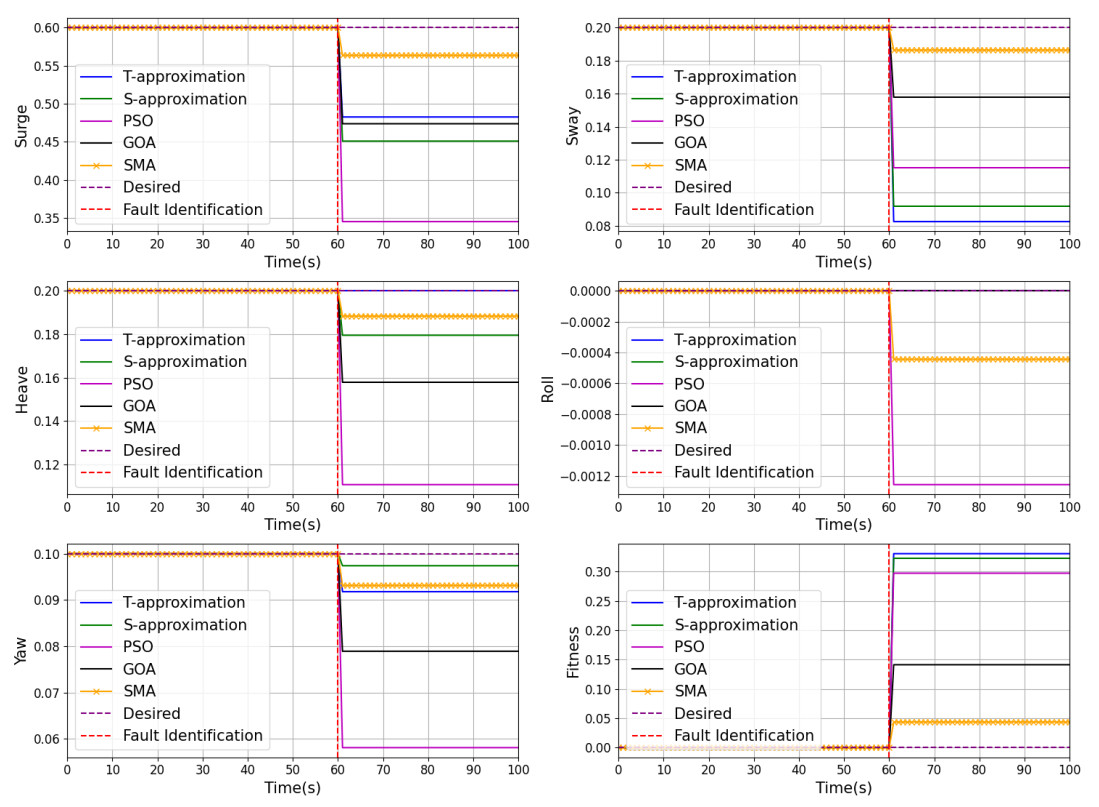
Figure 5. Multi-thruster reallocation problem for double-fault case.

4.3. Quadruple-fault case

The desired torque vector $$ \overline{\tau_d} $$ is also assigned as $$ [0.6, \ 0.2, \ 0.2, \ 0.0, \ 0.1] $$. At the 60-second mark, a catastrophic failure has significantly impacted the power distribution among all four thrusters. Specifically, the power output of $$ T1 $$ is reduced by 50%, $$ T2 $$ by 30%, $$ T3 $$ by 20%. The situation is more critical for T5, which has undergone a substantial 80% decrease in power, the corresponding $$ W=[0.5, \ 0.7, \ 0.8, \ 1.0, \ 0.2, \ 1.0] $$. This drastic power imbalance poses a formidable challenge to the overall functionality and stability of the vehicle. The obtained calculation results are shown in Table 3.

The pseudo-inverse solution $$ \overline{T} $$ is $$ [0.5933, \ 0.7933, \ 0.8067, \ 0.2067, \ 0.2, \ 0.2] $$ and three components are unfeasible because $$ {\overline{T}}_1>0.5, {\overline{T}}_2>0.7, {\overline{T}}_3>0.8 $$. Utilizing the T-approximation method, values exceeding control constraints are truncated. Specifically, 0.5933 will be set to 0.5, and 0.7933 will be set to 0.7, 0.8067 will be set to 0.8, so that $$ \overline{T} $$ is adjusted to $$ T^\ast=[0.5, \ 0.7, \ 0.8, \ 0.2067, \ 0.2, \ 0.2] $$, and the corresponding $$ \overline{\tau} $$=[0.3967, 0.1683, 0.12, -0.08, 0.0483]. Utilizing the S-approximation method, all the components times $$ {0.5}/{0.5933} $$, so that $$ \overline{T} $$ is adjusted to $$ T^\ast $$=[0.5, 0.6685, 0.6798, 0.1742, 0.1685, 0.1685], and the corresponding $$ \overline{\tau}=[0.359, \ 0.1469, \ 0.1011, \ -0.0674, \ 0.0379] $$.

Due to damage to the vertical thruster, both T-approximation and S-approximation lost control over the Heave and Roll axes, leading to increased errors and loss of effective submarine control [Figure 6]. Despite these challenges, PSO, GOA, and SMA corrected the direction error successfully. Notably, even in such difficult conditions, SMA managed to keep the magnitude error within 5%. This control strategy maintained the submarine’s direction without reducing its operational efficiency. SMA consistently delivered the best results in cases involving single-fault, double-fault, or quadruple-fault, demonstrating its potential as a reliable FTC method.

Figure 6. Multi-thruster reallocation problem for quadruple-fault case.

4.4. Efficiency and stability

This section compares the efficiency of the three algorithms: PSO, GOA, and SMA. Figure 7 illustrates the relationship between time and optimum fitness for three algorithms applied to thruster power redistribution under single-fault, double-fault, and quadruple-fault cases. Notably, after a large number of experiments, we found that the increase in the number of thruster failures does not significantly affect the running time of each algorithm. Therefore, the running times shown in the paper are the average results obtained from multiple times.

Figure 7. Runtime and fitness of PSO, GOA and SMA methods using the same operating parameters for different fault cases. PSO: Particle swarm optimization; GOA: grasshopper optimization algorithm; SMA: slime mold algorithm.

The results are displayed in Table 4. All operating parameters are consistent. Runtime represents the total duration required for the algorithm to complete 200 iterations, ensuring that all algorithms have fully converged after these iterations. Due to its simple structure, PSO achieves the fastest running speed at just 0.119 s. However, PSO consistently falls short in terms of accuracy across all fault conditions. GOA, on the other hand, exhibits strong performance in accuracy for both single and double-fault cases. Despite this, its slower speed, approximately 0.3 s, fails to meet the real-time requirements for FTC systems. Moreover, under the quadruple-fault case, the performance of GOA deteriorates significantly; a sharp increase in magnitude error makes it incapable of FTC. SMA may not match the speed of PSO, with a running time of 0.24 s, but it consistently delivers the best results across all cases, including extreme ones. These observations affirm the effectiveness of FTC in UUVs and underscore the superior adaptability of SMA under various fault cases.

Authors’ contributions

Wrote the PSO, GOA, and SMA programs and the draft: Zeng, T.

Organized the experiment and guided the work: Zhu, D.; Gu, C.; Simon, X. Y.

Availability of data and materials

Not applicable.

Financial support and sponsorship

None.

Conflicts of interest

Simon, X. Y. is the Editor-in-Chief of the journal Intelligence & Robotics, Zhu, D. is the guest editor of the Special Issue of “Updates in Underwater Robotics”, and Editorial Board Member of the journal Intelligence & Robotics, while the other authors have declared that they have no conflicts of interest.

Ethical approval and consent to participate

Not applicable.

Consent for publication

Not applicable.

Copyright

© The Author(s) 2025.

REFERENCES

1. Li, J.; Yang, G. Development and prospect of adaptive fault-tolerant control. Control. Decis. 2014, 29, 1921-26.
2. Li, Y.; Hou, Y.; Liu, C. Adaptive optimal fault-tolerant control based on fault degree. J. Comput. Eng. Appl. 2021, 57, 295-302.
3. Shen, Q.; Jiang, B.; Shi, P.; Lim, C. C. Novel neural networks-based fault tolerant control scheme with fault alarm. IEEE. Trans. Cybern. 2014, 44, 2190-201.
4. Shi, P.; Wang, X.; Meng, X.; He, M.; Mao, Y.; Wang, Z. Adaptive fault-tolerant control for open-circuit faults in dual three-phase PMSM drives. IEEE. Trans. Power. Electron. 2023, 38, 3676-88.
5. Kadiyam, J.; Parashar, A.; Mohan, S.; Deshmukh, D. Actuator fault-tolerant control study of an underwater robot with four rotatable thrusters. Ocean. Eng. 2020, 197, 106929.
6. Baraniuk, T.; Simoni, R.; Weihmann, L. Fault-tolerant architecture for AUVs. In: 2018 IEEE/OES Autonomous Underwater Vehicle Workshop (AUV), Porto, Portugal. Nov 06-09, 2018. IEEE, 2018. pp. 1-6.
7. Panda, J. P.; Mitra, A.; Warrior, H. V. A review on the hydrodynamic characteristics of autonomous underwater vehicles. J. Eng. Marit. Environ. 2021, 235, 15-29.
8. Yu, J.; Zhang, A.; Wang, X. Research on thruster fault tolerant control allocation of a 7000m manned submarine. Robot 2006, 28, 519-24.
9. Esna, A. A.; Khaki, S. A.; Yazdanpanah, M. J. Reconfigurable control system design using eigen structure assignment: static, dynamic and robust approaches. Int. J. Control. 2005, 78, 1005-16.
10. Lin, C. M.; Chen, C. H. Robust fault-tolerant control for a biped robot using a recurrent cerebellar model articulation controller. IEEE. Trans. Syst. Man. Cybern. B. 2007, 37, 110-23.
11. Conte, G. Underwater robots: motion and force control of vehicle–manipulator systems. Int. J. Adapt. Control. Signal. Process. 2004, 18, 603-4.
12. Yang, K. C.; Yuh, J.; Choi, S. K. Experimental study of fault-tolerant system design for underwater robots. In: Proceedings. 1998 IEEE International Conference on Robotics and Automation (Cat. No.98CH36146), Leuven, Belgium. May 20, 1998. IEEE, 1998; pp. 1051-6.
13. Yang, K. C. H.; Yuh, J.; Choi, S. K. Fault-tolerant system design of an autonomous underwater vehicle ODIN: an experimental study. Int. J. Syst. Sci. 1999, 30, 1011-9.
14. Zhang, Y.; Jiang, J. Bibliographical review on reconfigurable fault-tolerant control systems. Annu. Rev. Control. 2008, 32, 229-52.
15. Podder, T. K.; Sarkar, N. Fault tolerant decomposition of thruster forces of an autonomous underwater vehicle. In: Proceedings 1999 IEEE International Conference on Robotics and Automation (Cat. No.99CH36288C), Detroit, USA. May 10-15, 1999. IEEE, 1999; pp. 84-9.
16. Podder, T. K.; Sarkar, N. Fault-tolerant control of an autonomous underwater vehicle under thruster redundancy. Robotics. Auton. Syst. 2001, 34, 39-52.
17. Fossen, T. I. Guidance and control of ocean vehicles. 1994. https://books.google.com/books/about/Guidance_and_Control_of_Ocean_Vehicles.html?id=cwJUAAAAMAAJ. (accessed on 2025-03-19).
18. Omerdic, E.; Roberts, G. Thruster fault diagnosis and accommodation for open-frame underwater vehicles. Control. Eng. Pract. 2004, 12, 1575-98.
19. Zhao, W.; Liu, H.; Wan, Y. Data-driven fault-tolerant formation control for nonlinear quadrotors under multiple simultaneous actuator faults. Syst. Control. Lett. 2021, 158, 229-52.
20. Chen, H.; Jiao, S.; Heidari, A. A.; Wang, M.; Chen, X.; Zhao, X. An opposition-based sine cosine approach with local search for parameter estimation of photovoltaic models. Energy. Convers. Manag. 2019, 195, 927-42.
21. Chen, H.; Xu, Y.; Wang, M.; Zhao, X. A balanced whale optimization algorithm for constrained engineering design problems. Appl. Math. Model. 2019, 71, 45-59.
22. Wang, M.; Chen, H.; Yang, B.; et al. Toward an optimal kernel extreme learning machine using a chaotic moth-flame optimization strategy with applications in medical diagnoses. Neurocomputing 2017, 267, 69-84.
23. Wang, M.; Chen, H. Chaotic multi-swarm whale optimizer boosted support vector machine for medical diagnosis. Appl. Soft. Comput. 2020, 88, 105946.
24. Chen, M.; Liu, Y.; Zhu, D.; Shen, A.; Wang, C.; Ji, K. Parameter identification of an open-frame underwater vehicle based on numerical simulation and quantum particle swarm optimization. Intell. Robot. 2024, 4, 216-29.
25. Zhu, D.; Liu, J.; Yang, S. X. Particle swarm optimization approach to thruster fault-tolerant control of unmanned underwater vehicles. Int. J. Robot. Autom. 2011, 26.
26. Tian, Q.; Wang, T.; Liu, B.; Ran, G. Thruster fault diagnostics and fault tolerant control for autonomous underwater vehicle with ocean currents. Machines 2022, 10, 582.
27. Zhu, D.; Liu, Q.; Hu, Z. Fault-tolerant control algorithm of the manned submarine with multi-thruster based on quantum-behaved particle swarm optimization. Int. J. Control. 2011, 84, 1817-29.
28. Zhu, D. J.; Wang, L.; Hu, Z.; Yang, S. X. A grasshopper optimization-based fault-tolerant control algorithm for a human occupied submarine with the multi-thruster system. Ocean. Eng. 2021, 242, 110101.
29. Zhu, D. J.; Wang, L.; Zhang, H.; Yang, S. X. A GOA-based fault-tolerant trajectory tracking control for an underwater vehicle of multi-thruster system without actuator saturation. IEEE. Trans. Autom. Sci. Eng. 2024, 21, 771-82.
30. Sun, B.; Pang, W.; Chen, M.; Zhu, D. Development and experimental verification of search and rescue ROV. Intell. Robot. 2022, 4, 355-70.
Cite This Article
How to Cite
Download Citation
Export Citation File:
Type of Import
Tips on Downloading Citation
Citation Manager File Format
Direct Import: When the Direct Import option is selected (the default state), a dialogue box will give you the option to Save or Open the downloaded citation data. Choosing Open will either launch your citation manager or give you a choice of applications with which to use the metadata. The Save option saves the file locally for later use.
Indirect Import: When the Indirect Import option is selected, the metadata is displayed and may be copied and pasted as needed.
About This Article
Copyright
Comments
Comments must be written in English. Spam, offensive content, impersonation, and private information will not be permitted. If any comment is reported and identified as inappropriate content by OAE staff, the comment will be removed without notice. If you have any queries or need any help, please contact us at [email protected].