

Hot deformation behavior investigation of heat-resistant aluminum matrix composite based on Arrhenius model and machine learning
 0
0 Abstract
The heat-resistant aluminum matrix composite (AMC) exhibits excellent thermal performance due to the presence of heat-resistant dispersed nano-phases. Accurately characterizing high-temperature flow stress is essential for comprehending the mechanisms of deformation and improving material workability. To enhance the accuracy of modeling the flow stress for a new heat-resistant AMC during high-temperature processing, a set of isothermal compression tests at elevated temperatures was conducted. This testing was performed on the composite under varying temperature levels (473, 523, 573, 623, and 673 K) and distinct strain rates (0.001, 0.01, and 0.1 s-1). To accurately characterize the flow stress of the composite material at high temperatures, three distinct models were devised: (1) an Arrhenius model that includes strain compensation; (2) a back-propagation neural network (BPNN) model; and (3) a BPNN model optimized using a genetic algorithm (GA-BPNN). The strain compensation theory enhances the Arrhenius model’s ability to capture nonlinear characteristics, while the genetic algorithm (GA) optimizes the BPNN model’s parameter settings. The accuracy of each model in describing flow stress was compared to determine their effectiveness. The findings demonstrate that the GA-BPNN model achieved superior fitting accuracy, with a root mean square error (RMSE) of 6.48, accompanied by a coefficient of determination (R2) of 0.991 and a mean absolute error (MAE) of 5.4. To evaluate the generalization capabilities of the three models, a new data set was utilized for verification. The generalization capabilities of the three models were verified using a set of new data. The GA-BPNN model demonstrates outstanding generalization capability, achieving the highest prediction accuracy for new datasets, with R2 = 0.9102, RMSE = 9.09, and MAE = 7.83. Using the GA-BPNN model’s fitting results, a hot processing map was developed, and the optimal processing window (573 to 673 K) was identified. This study serves as a valuable reference for optimizing the processing parameters of heat-resistant AMCs and proposes a novel approach combining strain compensation and machine learning for high-temperature flow stress description. While the current framework demonstrates computational robustness, extending conclusions to composites with significantly different compositions requires further validation.

Keywords
INTRODUCTION
Due to their superior mechanical characteristics, aluminum matrix composites (AMCs) are extensively utilized in various industries, including aerospace, rail transportation, and electronics[1,2]. Recent studies demonstrate that the properties of AMCs can be significantly enhanced through in-situ fabrication methods. However, as technological advancements progress, there is a growing demand for these materials to fulfill more stringent performance requirements, particularly in heat resistance[3]. Unfortunately, the strength of AMCs significantly decreases with the rapid coarsening of the nanoprecipitates under elevated temperature service conditions[4]. To address this challenge, a high-volume fraction of dispersed heat-resistant nanoparticles can be incorporated to enhance the strength of AMCs at elevated temperatures[4-10]. However, this enhancement often compromises machinability due to the increased presence of hard reinforcing phases[11]. Consequently, optimizing the hot working process becomes critical to achieve a balance between mechanical performance and manufacturability[12].
The hot deformation behavior of AMCs involves several interrelated phenomena, such as dynamic recovery (DRV), dynamic recrystallization (DRX) and work hardening, which together contribute to the complexity of their mechanical properties[13]. Understanding the high temperature flow stress is essential, as it can provide insights into the underlying microscopic mechanisms governing these behaviors[14]. Accurately predicting flow stresses at elevated temperatures is crucial for understanding the behavior of AMCs during processing. To describe the hot deformation behavior of AMCs, constitutive equations are commonly utilized. Currently, these constitutive models can be classified into three categories: phenomenological, physical, and kinetic models[15]. Among them, phenomenological constitutive models, such as the Johnson-Cook (JC) model[16], the Bodner-Partom (BP) model[17], the Fields-Backofen (FB) model[18], and the Khan-Huang (KH) model[19], are characterized by their simplicity and require fewer parameters. However, they lack a solid theoretical foundation and fail to consider the impact of microstructural evolution on deformation. In contrast, physical constitutive models can explain the physical properties of materials but require the determination of more material parameters. The Zerilli-Armstrong model[20] and the mechanical threshold stress model[21] are widely recognized as classical models. The dynamic constitutive model was first introduced by Sellars and McTegart as the Arrhenius model[22]. This model not only describes the functional relationship among deformation parameters but also calculates various physical parameters related to deformation mechanisms. Due to its versatility, the Arrhenius model is extensively applied in the study of hot deformation behavior of composites. However, the high complexity of composite deformation at elevated temperatures results in low prediction accuracy of flow stress using traditional methods, limiting their applicability.
To address these limitations, researchers have increasingly utilized artificial neural networks (ANNs) in recent years to predict the relationship between flow stress and deformation parameters, achieving high prediction accuracy[23,24]. Among these networks, the back-propagation neural network (BPNN) is one of the most commonly used models[25-30]. However, it is important to note that the application of BPNN is constrained by issues such as the tendency to become trapped in local optima and significant dependence on initial weights and biases[31]. The introduction of GAs can help obtain optimal weights and thresholds of the BPNN model, thereby enhancing the model’s stability and accuracy. Consequently, GA-optimized BPNN (GA-BPNN) models exhibit improved global search capability and generalization performance[32]. For example, Huang et al. established a GA-BPNN approach to predict the load-displacement hysteresis curve of a diaphragm joint under low-cycle cyclic loading[33]. Compared to BPNN model, the GA-BPNN model yielded higher accuracy. Similarly, Zhu et al. utilized the Arrhenius model and the BPNN framework to describe hot deformation behavior and established an improved BPNN model optimized via GAs[34]. Their results showed a correlation coefficient between the predicted and experimental values of 99.99%, with an average absolute relative error of only 0.54%. The GA-BPNN model produced more accurate predictions compared to traditional algorithms. Despite these promising developments, research focusing on the application of GA-BPNN models to the hot deformation behavior of novel heat-resistant AMCs remains relatively limited.
This research has developed a novel heat-resistant AMC containing a substantial amount of heat-resistant Al–O nanostrips, significantly enhancing the composite’s mechanical properties at elevated temperatures. However, the hot deformation behavior of this composite has not been extensively researched, particularly regarding its mechanisms and implications under various processing conditions. This paper presents a GA-BPNN model designed to characterize the flow stress occurring during the composite’s hot deformation process. We established Arrhenius, BPNN, and GA-BPNN models to describe the composite’s hot deformation behavior and compared the fitting results of three models to get the accuracy of the GA-BPNN model. The generalization capabilities of the three models were verified using a set of new data. The flow stress obtained from the GA-BPNN model was used to create a hot processing map, and the deformed composite’s microstructure analysis was conducted to validate the accuracy of the hot processing map. This study is expected to provide valuable references for the formulation of hot processing parameters for this novel heat-resistant AMC in practical production settings and offer a machine-learning approach for describing flow stress in these composites. However, its adaptability under various conditions requires further testing to enhance generalizability.
MATERIALS AND METHODS
Material preparation
Pure aluminum powder (Shanpu Chemical Co., Ltd., Shanghai, China) with an average particle size of 10 μm was used as the starting material to prepare the composite. The aluminum powder was ball-milled using planetary ball milling (ND8-4L, Nanjing Nanda Tianzun Electronics Co., Ltd., China) with 1-liter stainless steel vials and 1 kg of stainless steel balls as the milling media. Milling took place in an argon environment. The process was carried out at a speed of 210 rpm over a duration of 30 h, with a 15:1 ball-to-powder mass ratio set. Moreover, 10 wt.% ethanol was added into the aluminum powder as the process control agent. The milled powder was sealed into the graphite die inside the glove box and then consolidated at 893 K and
Microstructure characterization
Microstructures of the obtained composite were characterized using field emission scanning electron microscopy (SEM, Sigma500, ZEISS, Germany) with electron backscatter diffraction (EBSD, Octane Elite Ultra, EDAX, USA) and transmission electron microscopy (TEM, JEM-2100F, JEOL, Japan). The phase of the nanocomposite was analyzed by an energy dispersive spectrometer (EDS, OXFORD, X-Max80, UK) and X-ray diffraction (XRD, PANalytical, Empyrean, Netherlands).
Figure 1A illustrates the SEM images of representative composites. The images reveal a significant presence of nanostrips evenly distributed within the matrix. The nanostrips have a width of about 10 nm, and their average length is about 180 nm. The volume fraction of these nanostrips is estimated as 12% from the SEM images by ImageJ software. Figure 1B displays EBSD images of the composite, indicating that the grains of the aluminum matrix exist at the nanoscale. Figure 1C shows that the material mainly contains Al, with a small amount of Al4C3. Figure 1D indicates that the nanostructures in the matrix primarily contain O, and the quantitative analysis of the energy spectrum surface scan also shows that the content of O is greater than that of C. Therefore, we preliminarily conclude that most of our nanostrips are Al–O structures. The absence of characteristic peaks for Al–O nanostrips in the XRD results may be attributed to the extremely small size of the nanostrips. Further detailed structural characterization will be presented in future work.

Figure 1. (A) Typical SEM image of composite; (B) Typical EBSD image of composite; (C) Typical XRD image of composite; (D) Typical EDS image of composite. SEM: Scanning electron microscopy; EBSD: electron backscatter diffraction; XRD: X-ray diffraction; EDS: energy dispersive spectrometer.
The formation of Al4C3 is likely due to the reaction of carbon introduced during processing with Al at elevated temperatures. The high content of Al–O nanostructures may result from the reaction between anhydrous ethanol and the aluminum matrix during ball milling and hot pressing, despite the use of inert atmospheric conditions.
Compression test
Compression tests were conducted at strain rates of 0.001, 0.01, and 0.1 s-1, and at temperatures of 473, 523, 573, 623, and 673 K. Each condition was tested three times using a testing machine (MTS, Instron 2367 equipped with a heating furnace, Instron, USA), with cylindrical specimens measuring 4 mm in height and 2 mm in diameter. All test specimens were prepared using a wire-cut electrical discharge machining (WEDM, Jiangsu Founder CNC Machine Tool Co., Ltd, DK7735, China), ensuring geometric accuracy within ± 0.01 mm. The specimens were gradually heated to the specified temperature, increasing at a rate of 10 °C per minute and held for 10 min to ensure uniform thermal conditions. Stress-strain curves were then derived from the force-displacement data.
Arrhenius model
The hot deformation behavior of composites is governed by thermally activated processes, which can typically be described using the Arrhenius-type equation[22]. This equation relates flow stress, strain rate, and deformation temperature during the hot deformation process. It is particularly useful for understanding how the material responds under different thermal and mechanical conditions.
For different stress levels, the Arrhenius model can be adapted as follows. When the material is under low stress, the flow stress and strain rate follow a power-law relationship:
For higher stress levels, the model is adjusted to reflect the impact of stress on material’s flow behavior, which is usually expressed as:
Finally, to account for all stress levels, the model can be generalized using
which incorporates hyperbolic sine function to describe strain rate’s dependence on flow stress. A and A1 are structural factors,
Additionally, Zener and Hollomon[35] showed that the flow stress is affected by temperature and strain rate, which can be effectively described using a temperature-compensated strain rate factor. This parameter, known as the Zener-Hollomon parameter (Z), can be incorporated into the Arrhenius equation as follows:
The Z parameter is particularly useful for characterizing deformation processes because it allows for the comparison of deformation conditions at different temperatures and strain rates.
Database establishment of neural network
To ensure both diversity and reliability of the dataset, a wide range of testing conditions was considered as the input features, including:
(1) Temperature: The testing temperature of the sample, expressed in degrees Fahrenheit (K).
(2) Strain Rate: The rate at which strain is applied, expressed in inverse seconds (s-1).
(3) Strain: A measure of the amount of deformation, typically expressed as a percentage without units.
The output target is the flow stress (τ), measured in megapascals (MPa), which indicates the material’s resistance to deformation under specific conditions. The flow stress is derived from the experimental stress-strain curves and is crucial for analyzing material performance and determining optimal processing parameters. It is important to note that these input features and output targets are consistent across all subsequent models in this study.
These conditions were carefully selected to capture the hot deformation behavior of the composite comprehensively. The temperature range was from 473 to 673 K, the strain rates were set at 0.001, 0.01, and 0.1 s-1, and the strain ranged from 0.05 to 0.2. A total of 1,500 datasets were collected from the experimental flow stress-strain curves, consisting of 100 strain values, three strain rates, and five temperatures.
To enhance model convergence and training efficiency, the raw data is normalized prior to the training process, ensuring that it falls within the range of 0 to 1, as determined by:
where Xi represents the original data, Xmin indicates the minimum value of the dataset, and Xmax signifies the maximum value of the dataset. Normalization reduces the influence of varying magnitudes of input variables, ensuring that all features contribute equally during training.
The normalized dataset was split into two segments: 80% was allocated for training the neural network, and the remaining 20% was used as a test set to assess the network’s performance.
To quantify predictive accuracy, the mean absolute error (MAE), the root mean square error (RMSE), and the coefficient of determination (R2) were introduced to assess the models’ performance. These metrics provide complementary understanding of the model’s effectiveness, with R2 reflecting proportion of variance explained, RMSE quantifying the average deviation magnitude, and MAE capturing the absolute prediction error. These metrics are given below:
Here n represents the sample’s number, yi stands for the i-th samples’ true value,
BPNN
The BPNN functions in two key phases: forward and backward propagation. In the forward phase, input data is processed through layers to produce output signals. When the output deviates from the target, the network initiates back-propagation, redistributing the error to adjust weights and thresholds. This continuous adaptation improves the network’s accuracy in predicting flow stress[25].
The BPNN architecture used in this study includes an input layer, an output layer, and a hidden layer composed of several interconnected neurons, as illustrated in Figure 2. The input layer comprises three nodes representing temperature, strain rate, and strain. The hidden layer includes 15 neurons, which were selected based on empirical testing to balance model complexity and accuracy. The activation function selected for the hidden layer is the hyperbolic tangent sigmoid function, whereas the output layer utilizes a linear transfer function. The parameters for the BPNN include a maximum iteration count of 100, a target error of 0.0001, a learning rate of 0.5, and 15 neurons in the hidden layer. These parameters were chosen based on preliminary experiments to ensure stable convergence and high accuracy. After establishing the model, a set of independent data is input for predicting the flow stress.

Figure 2. Model based on BPNN. BPNN: Back-propagation neural network.
GA
In a BPNN, the weight parameters and activation functions are critical factors influencing performance. The output produced by any individual neuron can be determined using
where n represents the number of input nodes, xi stands for the input vector, g refers to the activation function, wi denotes the weight vector, bi indicates the bias, and y signifies the output. For each computation, the error signal, representing the difference between experimental and predicted values, is propagated backward to modify the weights. If the initial weights and thresholds are poorly chosen, the training process may become stuck in local minima, preventing the model from reaching the global minimum of the error function. To enhance the accuracy of the model, this study employs a GA to optimize the BPNN.
The GA begins with a population of individuals, each representing a potential solution to an optimization problem. Each individual is a chromosome containing genes that determine its phenotype. The algorithm evolves the population through generations based on natural selection principles, yielding increasingly effective solutions.
Individuals are selected according to their fitness, and genetic operations such as crossover and mutation create a new population with innovative solutions. This iterative process enhances adaptation, resulting in the best individual of the final generation representing a near-optimal solution to the problem. Based on this approach, a more stable GA-BPNN model has been established, with the structure illustrated in Figure 3. The configuration of the BPNN model is consistent with the previous discussion. After adjustments, the final parameters for the GA are as follows: 2,000 training epochs, learning rate of 0.01, momentum factor of 0.01, target training error of 0.0001, population size of 30, number of evolution iterations of 50, and mutation and crossover probabilities of 0.2 and 0.8. After establishing the model, a set of independent data was input to describe the flow stress.

Figure 3. Schematic diagram of the GA-BPNN model structure. GA-BPNN: Genetic algorithm-optimized back-propagation neural network.
The hot processing map
The ability of the composite for plastic deformation and its assistance in identifying regions of flow instability can be reflected by the hot processing map. It serves as a vital research tool in the field of plastic forming. A widely utilized approach for constructing such a map is the dynamic materials model (DMM) proposed by Prasad et al.[36]. It integrates power dissipation map with instability map to identify the optimal parameter window for hot processing of composites. The input energy P of the system can be split into two parts: the dissipative quantity and the cooperative dissipative quantity:
Here, G is the energy dissipated as heat during plastic deformation. This energy arises from irreversible processes such as dislocation motion and lattice friction and contributes little to microstructural evolution. The symbol J represents the energy expended in altering the microstructure during the deformation process, such as DRX, grain boundary migration, and dislocation annihilation. This component is critical for understanding microstructural changes under specific processing conditions.
The distribution between G and J is governed by m (strain rate sensitivity index), defined as:
Under standard conditions, m’s value exhibits a nonlinear relationship with strain rate and temperature. In the case of viscoplastic solids, m’s value ranges between 0 and 1. As the m value increases, microstructural dissipation also increases. When m approaches zero, the energy dissipation is primarily dominated by G, with minimal contribution from J. This condition is often observed in scenarios involving dislocation pile-up and shear localization, which can limit the extent of microstructural evolution. Conversely, when m approaches one, the energy dissipation shifts towards J, potentially promoting DRX and a more uniform grain structure. These mechanisms are associated with improved material stability and deformation homogeneity.
Assuming that the material follows the constitutive equation:
The cooperative dissipative quantity J can be derived as:
When m = 1, the dissipation co-energy J attains its peak value.
The dissipation efficiency factor η, defined as:
provides a dimensionless measure of how effectively the energy is utilized for microstructural evolution. The dimensionless parameter η generally reflects the deformation mechanisms exhibited by materials under particular conditions of temperature and strain rate. High η values often correspond to regions of DRX, while low η values tend to indicate shear localization or other instability mechanisms. A power dissipation diagram can be developed by illustrating how the parameter η changes with strain rate and temperature.
Prasad et al. introduced an instability criterion derived from the principle of maximum irreversible thermodynamics, specifically for extensive plastic flow in continuous media[37]. The instability occurs when:
Here, D represents the dissipation function, which characterizes the material’s constitutive behavior and is derived from the dissipated power. According to the principle of the DMM, the cooperative dissipation quantity J can substitute the dissipation function D. Thus, the instability criterion becomes:
Then, we can obtain
According to the cooperative dissipative quantity J expressed in Equation (14), we obtain
From Equations (18) and (19), we can introduce an instability parameter ξ(
When ξ(
By plotting the ξ values on the two-dimensional plane of T vs. ln
RESULTS AND DISCUSSION
Flow behavior
Figure 4 illustrates the true stress vs. true strain curves for the composite material under different temperatures and loading rates. Under quasi-static loading conditions, the composite exhibits a strength of up to 400 MPa at 473 K. When the temperature rises to 673 K, strength remains approximately 200 MPa. Figure 5 depicts the correlation between temperature and peak stress, indicating that peak stress decreases as the deformation temperature increases, while it increases with higher strain rates.

Figure 4. Curves of true stress vs. true strain under various strain rates and temperatures during compression: (A) strain rate of 10-1; (B) strain rate of 10-2; (C) strain rate of 10-3.

Figure 5. The correlation between temperature and peak stress.
In Figure 4, the stress exhibits a rapid increase shortly after loading commences, which can be attributed to the abrupt rise in dislocation density induced by external forces, leading to a phenomenon known as work hardening. After the maximum flow stress is achieved, the stress-strain curve gradually declines and eventually stabilizes. This decline is attributed to the diminishing strengthening effect of the nanostrips. At higher temperatures, mechanisms of softening, including DRX and DRV, interact with hardening processes such as strain hardening. Once peak stress is reached, the softening mechanisms prevail, resulting in a gradual reduction in the stress-strain curve. Ultimately, the interaction between the softening and hardening mechanisms nearly balances out, leading to a stable stress-strain response[38]. As shown in Figure 5, an analysis comparing peak stress values at various strain rates demonstrates that the composite shows sensitivity to strain rate changes. Specifically, at a constant deformation temperature, an increase in strain rate corresponds to an increase in peak stress. This phenomenon occurs because higher strain rates accelerate dislocation movement, resulting in the production of relatively large deformations over shorter time intervals, which in turn leads to significant dislocation pile-up. The substantial increase in dislocation density raises the critical shear stress during deformation[39]. Additionally, the increased strain rate results in a shorter deformation time, hindering DRV and DRX[40,41]. This rapid deformation not only accelerates dislocation movement but also increases the likelihood of localized stress concentrations around the reinforcing phases. As the strain rate rises, the matrix experiences rapid plastic deformation, while the reinforcing phases may not deform at the same rate due to their different mechanical properties. This discrepancy creates a situation where the reinforcing phases can act as stress concentrators, exacerbating the non-uniform distribution of stress within the matrix[42-44]. The presence of these stress concentrations can lead to localized yielding in the matrix, which further complicates the overall deformation behavior. Consequently, the matrix’s ability to undergo plastic deformation is significantly impeded by the presence of the reinforcing phases.
In contrast, maintaining a constant strain rate while raising the temperature results in a reduction in peak stress. This reduction is attributed to enhanced thermal motion of atoms at higher temperatures, which increases dislocation mobility and weakens the work hardening and dislocation pile-up within the matrix. Several strengthening mechanisms are also diminished at elevated temperatures, such as the reduced effectiveness of grain refinement due to grain growth and the decreased interfacial bonding strength between the reinforcing phases and the matrix. This reduction in bonding strength results in a diminished capacity of the matrix to transfer loads to the particles, significantly lowering the shear resistance encountered by the particles. Furthermore, the rise in temperature can intensify the DRV and DRX processes within the matrix, ultimately resulting in a decrease in flow stress.
It is worth noting that at a loading rate of 10-3 s-1, we observed a significant decrease in the experimental curves (black and red lines) in the final sections at temperatures of 473 and 523 K. This corresponds to the material failure stage (e.g., crack propagation, interfacial peeling, or local necking), which occurs outside of the steady-state deformation state. The work in this paper is mainly focused on describing the steady-state flow behavior, so all subsequent models do not take into account the failure stage. We selected a strain range of 0.05 to 0.2. This choice ensures that our analysis focuses on the steady-state flow behavior and is not influenced by the failure stage.
Arrhenius model
In this chapter, we will derive the Arrhenius equation to elucidate the relationship between strain rate stress and temperature. Taking the logarithm of Equations (1)-(4) results in
By substituting the peak stress at a strain of 0.1 and the corresponding strain rate into Equations (21) and (22), and applying linear regression using the least squares method, we obtain the linear relationships between ln

Figure 6. (A) The correlation between ln
At a fixed strain rate, taking the partial derivative of Equation (23) with respect to (1/T) and rearranging gives activation energy’s expression:
The linear relationships between ln[sinh(ασ)] and (1/T) as well as ln[sinh(ασ)] and ln

Figure 7. (A) The correlation between ln[sinh(ασ)] and (1/T); (B) The correlation between ln[sinh(ασ)] and ln
The parameter Z reflects the relationship between the strain rate and activation energy, as given in Equation (24). By graphing ln(Z) vs. ln[sinh(ασ)], the accuracy of the analysis can be validated, as depicted in Figure 8. Furthermore, the intercept yields the value of ln(A). Thus, we can obtain the value of A as 1.67 × 10²⁰. The value of n = 23.1 can be determined from the curve’s slope. The correlation of correlation R2 for lnZ and ln[sinh(ασ)] exceeds 0.95.

Figure 8. The correlation between ln(Z) and ln[sinh(ασ)].
Finally, the derived constitutive equation for hot deformation, encompassing all conditions, is expressed as:
where A = 1.67 × 10²⁰, α = 3.28 × 10⁻³, n = 23.1, R = 8.31 J/(mol·K), and Q = 269.93 kJ/mol.
Although the Arrhenius model successfully derives the constitutive equation, it overlooks the equally important strain parameters. The activation energy for deformation and the constants are greatly affected by strain. Consequently, integrating strain parameters into the Arrhenius equation is crucial. In the strain range of 0.05 to 0.2, values are sampled at intervals of 0.025, and the material constants in Equation (29) are calculated for each corresponding strain value. The variation of constants with strain is depicted in Figure 9. Additionally, we represent the constants α, n, Q, and lnA at different strains using a fifth-degree polynomial, as given in
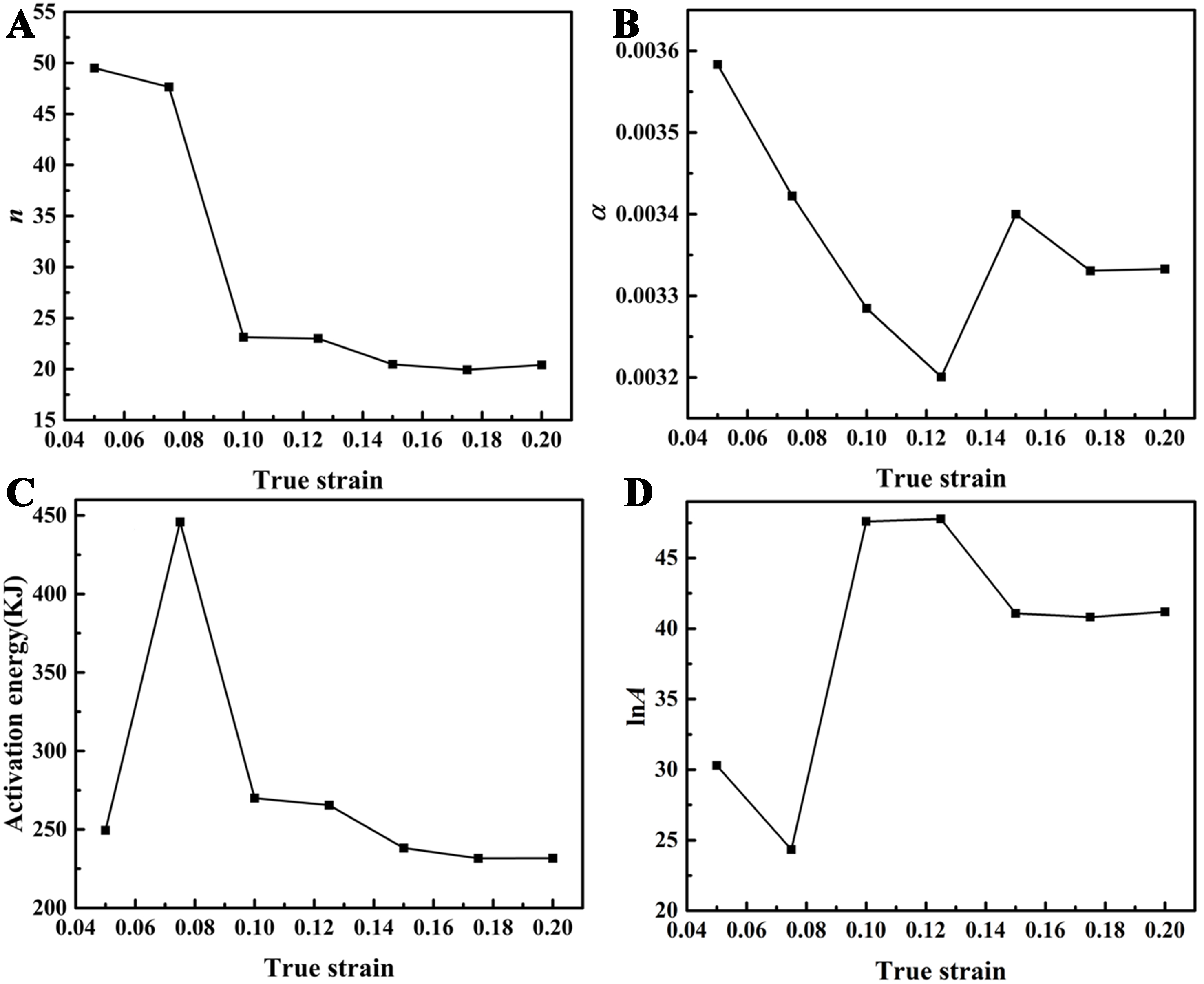
Figure 9. The relationship between material constants and true strain.
Then, we determine the coefficients of these equations through fitting, with the coefficients’ values presented in Table 1.
Coefficients of Equations (27)-(30)
| n | α | lnA | Q (kJ/mol) |
| n 0 = -5.50 × 10² | α 0 = -1.70 × 10⁻³ | A 0 = 8.56 × 10² | Q 0 = -7.12 × 10³ |
| n 1 = 3.02 × 10⁴ | α 1 = 2.81 × 10⁻¹ | A 1 = -4.08 × 10⁴ | Q 1 = 3.49 × 10⁵ |
| n 2 = -5.58 × 10⁵ | α 2 = -5.46 | A 2 = 7.39 × 10⁵ | Q 2 = 6.22 × 10⁶ |
| n 3 = 4.98 × 10⁶ | α 3 = 4.82 × 101 | A 3 = 6.07 × 10⁶ | Q 3 = 5.03 × 10⁷ |
| n 4 = -1.96 × 10⁷ | α 4 = -1.97 × 10² | A 4 = 2.03 × 10⁷ | Q 4 = -1.94 × 10⁸ |
| n 5 = 3.02 × 10⁷ | α 5 = 3.06 × 10² | A 5 = -4.02 × 10⁷ | Q 5 = 2.96 × 10⁸ |
After calculating the material constants, the established strain-compensated constitutive equation can yield flow stress values at different strains. By calculating values within a strain range of 0.05 to 0.2 at intervals of 0.025, both experimental and model-derived flow stress values were compared. Figure 10 illustrates the comparison between experimental data and model-derived values. The model-derived values closely align with the experimental findings obtained at strain rates of 10-3. At high strain rates, the material’s response becomes more complex due to rapid deformation processes. The strain-compensated Arrhenius model may not fully capture the interplay between work hardening and softening mechanisms (such as DRV and recrystallization) that dominate at these rates.

Figure 10. Flow stress experimental values and model-derived values at different strain rates based on the strain-compensated Arrhenius equation: (A) 10-1; (B) 10-2; (C) 10-3.
ANN model
BPNN model
The BPNN model was utilized to describe the flow stress during the hot deformation process. By calculating flow stress values within a strain range of 0.05 to 0.2 at intervals of 0.025, the experimental and model-derived values were compared. The outcomes, as illustrated in Figure 11, demonstrate that the BPNN produces accurate flow stress values across different conditions, including temperature, strain rate, strain, and other processing parameters.
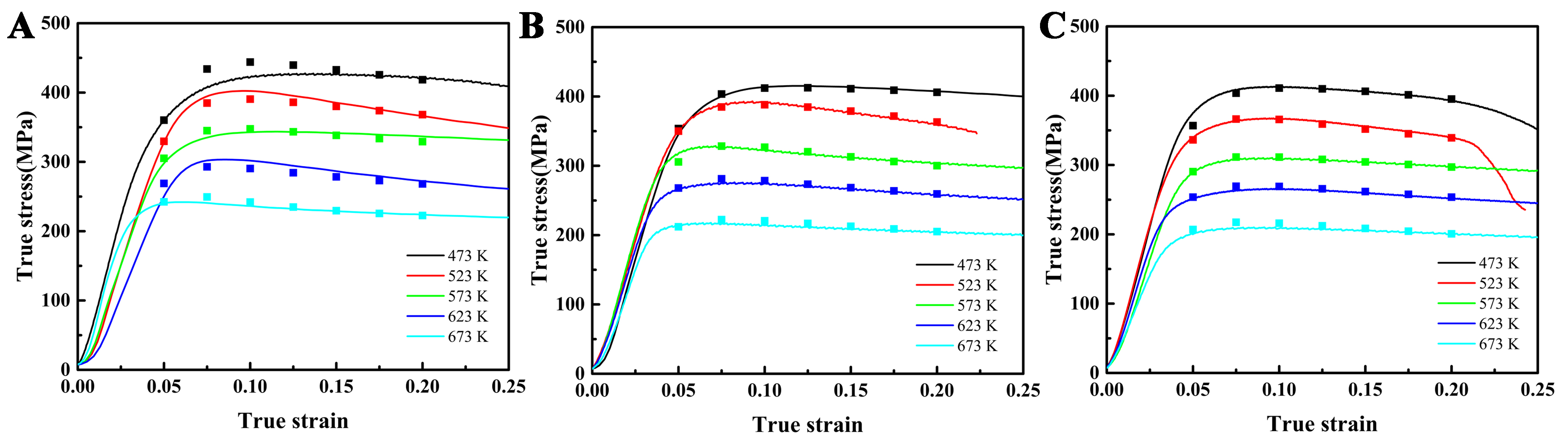
Figure 11. Model-derived flow stress values generated from the BPNN model with experimental values at different strain rates: (A) 10-1; (B) 10-2; (C) 10-3. BPNN: Back-propagation neural network.
GA-BPNN model
The flow stress was characterized using the GA-BPNN model. By calculating values of flow stress within a strain range of 0.05 to 0.2 at intervals of 0.025, the experimental and model-derived values were compared. The results are presented in Figure 12, where it is evident that the difference between values derived from the GA-BPNN model and those obtained experimentally is minimal.

Figure 12. Comparison of model-derived flow stress values obtained from the GA-BPNN model with experimental values at different strain rates: (A) 10-1; (B) 10-2; (C) 10-3. GA-BPNN: Genetic algorithm-optimized back-propagation neural network.
Comparison of accuracy among different models
Figure 13 illustrates a comparison of the experimental values and the model-derived values from the three models under different deformation conditions. From the figure, it is evident that at a strain rate of

Figure 13. Comparison of experimental values and model-derived values from three models at different strain rates: (A) 10-1; (B) 10-2; (C) 10-3.
Figure 14 illustrates the relationship between the values derived from the model and the experimental values obtained through comparison of three models. The R2 value for the GA-BPNN model exceeds that of other models, suggesting that GA-BPNN model provides a more accurate representation of the relationship between the experimental and model-derived values.

Figure 14. Comparison of model-derived values and experimental values from different models: (A) Training set of GA-BPNN model; (B) Testing set of GA-BPNN model; (C) Training set of BPNN model; (D) Testing set of BPNN model; (E) Arrhenius model. GA-BPNN: Genetic algorithm-optimized back-propagation neural network.
The R2, RMSE, and MAE values for the model-derived values of the testing and training sets from the three models are shown in Table 2.
Comparison of R2, RMSE, and MAE among different models
| Model | R 2 | MAE | RMSE |
| Arrhenius data | 92.12% | 17.19 | 21.43 |
| BPNN testing data | 99.02% | 5.47 | 6.78 |
| BPNN training data | 99.09% | 5.44 | 8.78 |
| GA-BPNN testing data | 99.11% | 5.40 | 6.48 |
| GA-BPNN training data | 99.15% | 5.43 | 8.49 |
The GA-BPNN model demonstrated remarkable predictive accuracy and stability in this study. Specifically, the R2 value for the testing set reached 99.11%, while that for the training set was 99.15%, indicating a high capability for explaining the variability of the target variable. The model also exhibited superior performance in terms of RMSE and MAE metrics, with a testing set RMSE of 5.40 and MAE of 6.48, as well as a training set RMSE of 5.43 and MAE of 8.49. These values are lower than those of the comparative models, highlighting the ability of GA-BPNN to provide more precise predictions, particularly in the context of complex data. Furthermore, the proximity of errors between the training and testing sets suggests that the model possesses good stability.
Furthermore, by comparing the predictive accuracy (R2 values) of different aluminum-based materials during hot deformation (as shown in Table 3), it is evident that machine learning models, particularly BPNN and GA-BPNN, demonstrate significant advantages in accuracy. In contrast, the precision of traditional Arrhenius models is notably lower than that of the machine learning approaches. Furthermore, the accuracy achieved in this study is comparable to that of similar research. Overall, both GA-BPNN and BPNN models exhibit higher precision and stability in predicting the hot deformation of aluminum-based materials, particularly when addressing complex materials, thereby validating their superiority and potential for application.
Comparative analysis of R2 values for different hot deformation models in aluminum-based materials
| Materials | Model | R 2 | Ref. |
| Al-Mg alloys | BPNN | 99.79% | [24] |
| Al-Zn-Mg-Cu-Zr alloys | BPNN | 99.73% | [26] |
| Al-Cu-Mg-Ag alloys | BPNN | 99.64% | [27] |
| Al-Cu-Mg-Ag alloys | Arrhenius model | 97.62% | [27] |
| Al-Cu-Mg-Pb alloys | BPNN | 99.90% | [28] |
| Al-Cu-Mg-Pb alloys | Arrhenius model | 98.50% | [28] |
| Al-Cu-Mg-Pb alloys | Strain-compensated Arrhenius model |
99.20% | [28] |
| Al-Cu-Mg-Pb alloys | JC model | 97.60% | [28] |
| Al-Zn-Mg-Mn-Zr alloys | BPNN | 99.83% | [29] |
| Al-Zn-Mg-Cu alloys | GA-BPNN | 99.98% | [30] |
| Al-Zn-Mg-Cu alloys | Strain-compensated Arrhenius model |
98.74% | [30] |
| Al matrix composite | GA-BPNN | 99.11% | This work |
| Al matrix composite | BPNN | 99.02% | This work |
| Al matrix composite | Strain-compensated Arrhenius model |
92.12% | This work |
The high precision of our BPNN and GA-BPNN models can be attributed to several critical factors that enhance their predictive accuracy. Firstly, the feature selection process focuses on three essential input parameters that are crucial for capturing the thermal deformation behavior of aluminum-based materials. The BPNN architecture, consisting of an input layer, one hidden layer with 15 neurons, and an output layer, strikes an optimal balance between complexity and accuracy. Additionally, the use of the GA for optimizing the BPNN parameters enhances performance significantly. The GA explores a diverse solution space and converges on optimal weights for the neural network. Overall, the combination of effective feature selection, a well-structured BPNN architecture, and a robust optimization approach through GA leads to the high predictive accuracy of our models, showcasing their innovation and strong applicability in predicting flow stress in aluminum-based materials.
Generalization ability of different models
Generalization ability is a core concept in machine learning, referring to a model’s capacity to make predictions on unseen new data. If a model performs well on the training set and possesses strong generalization ability, it can not only achieve excellent results on the training data but also maintain that level of performance on new, unknown data. This capability is crucial for ensuring prediction accuracy in practical applications. Therefore, models with strong generalization ability can adapt more effectively to new information, providing more reliable predictive outcomes.
To evaluate the generalization ability of the model, we performed compression tests at two temperatures, 723 and 773 K, utilizing a strain rate of 10-3. This enabled us to obtain the high-temperature compression mechanical curves for the material. We selected points at intervals of 0.025 within the strain range of 0.05 to 0.2, utilizing the material’s strain rate, strain and temperature as feature inputs for the Arrhenius, BPNN, and GA-BPNN models. The predicted values from these three models were then compared with the actual curves, as illustrated in Figure 15. The accuracy metrics for the predicted values from the three models, including MAE, R2, and RMSE, are presented in Table 4.

Figure 15. Comparison between the experimental data and the predicted values generated by various models on the validation: (A) Data of 723K; (B) Data of 773 K.
Comparison of R2, RMSE, and MAE among different models
| Model | R 2 | MAE | RMSE |
| Arrhenius | -92.98% | 36.91 | 42.14 |
| BPNN | 35.81% | 21.87 | 24.31 |
| GA-BPNN | 91.02% | 7.83 | 9.09 |
It is evident that the predictions made by the GA-BPNN model align more closely with the actual values, showcasing a higher level of accuracy. This finding suggests that the GA-BPNN model exhibits strong generalization capacity, allowing it to accurately characterize the high-temperature flow stress of this heat-resistant AMC material.
Hot processing map based on the stress obtained from GA-BPNN model
To determine the appropriate hot processing parameters for the composite, we employed the stress value get from the GA-BPNN model to create hot processing map. It is crucial to select strain points at which the material flow remains relatively stable in order to effectively capture the behavior during the hot processing. The flow stress values that correspond to a true strain of 0.2 are selected from the data obtained from the GA-BPNN model to construct a hot processing map.
In the two-dimensional plane of temperature vs. strain rate, connecting points with the dissipation rate η produces contour lines for η, which constitute the power dissipation map, as shown in Figure 16A. The η is calculated by Equations (12)-(15).

Figure 16. (A) Power dissipation map (η); (B) Instability map (ξ); (C) Hot processing map of the composite.
By plotting the ξ values on the two-dimensional plane of T vs. ln
Microstructure verification of hot processing map
To assess the precision of the established hot processing map, we characterized the microstructure of both the flow instability region and the flow stability region. Figure 17 presents the SEM images of the composite after deformation under different conditions. At 473 K, voids and cracks were observed at various strain rates. In contrast, at higher temperatures, the applied deformation localized in specific regions, leading to the development of distinct shear bands. The composite exhibited enhanced flow ability at elevated temperatures, significantly reducing the incidence of cracks and creating more favorable conditions for the hot processing of the composite.

Figure 17. SEM images of deformed samples under different conditions: (A) 473 K/10-1; (B) 473 K/10-2; (C) 473 K/10-3; (D) 573 K/10-1; (E) 573 K/10-2; (F) 573 K/10-3; (G) 673 K/10-1; (H) 673 K/10-2; (I) 673 K/10-3. SEM: Scanning electron microscopy.
Furthermore, we conducted TEM characterization under the temperature of 673 K and a strain rate of 10-3 in the hot stable processing region and compared it with the original sample, as shown in Figure 18. After hot deformation, the size of the nanostrips remained largely unchanged, with no significant cracks or voids observed. The interface between the nanostrips and the matrix remained well-bonded and clean, with no visible segregation at the grain boundaries and no significant additional phases formed. Additionally, the aluminum grains did not show abnormal growth, as illustrated in Figure 19. In summary, the composite exhibits good microstructural stability during deformation at elevated temperatures, contributing to the stability of the composite’s deformation.

Figure 18. Microstructural images of the composite before and after deformation at a strain rate of 10-3 and temperature of 673 K: (A-C) show the state before deformation, while (D-F) illustrate the condition after deformation.

Figure 19. Statistical analysis of grain size of the composite before and after hot deformation: (A) before deformation; (B) after deformation.
CONCLUSIONS
This study investigated the elevated temperature deformation behavior of novel heat-resistant AMCs under varying strain rates and temperatures. The following conclusions can be made:
(1) Flow stress equation: Flow stress equation for the composite was derived based on the Arrhenius model through a kinetic analysis of the experimental curves. A strain-compensated Arrhenius model was developed to incorporate the effects of strain on the model-derived flow stress of the material. This approach facilitated the determination of key material parameters, including a stress exponent of 23.1 and an activation energy of 269.93 kJ/mol.
(2) Data-driven flow stress modeling: Flow stress of the heat-resistant AMCs was described using strain-compensated Arrhenius models, BPNN models, and GA-BPNN models. GA-BPNN models achieved the highest agreement with experimental data, demonstrating a correlation coefficient of R2 = 0.9911. We also tested the generalization capabilities of three models using new data. The GA-BP model performed the best, showing strong generalization abilities. It achieved prediction accuracy with an R2 value of 0.9102. These results indicate that the GA-BPNN model not only works well with training data but also performs reliably with new data. Thus, the GA-BPNN model is the most effective among those we tested and has significant practical value.
(3) Optimal processing parameters: Based on the values of flow stress calculated by the GA-BPNN model, the stable deformation region established from the hot processing map was T = 573-673 K. Corresponding structural characterization under these conditions was validated through SEM and TEM analysis, confirming the accuracy of the hot processing map.
This study demonstrates that the GA-BPNN model exhibits excellent performance in predicting the elevated temperature deformation behavior of heat-resistant AMCs. However, its applicability to other material systems has not been examined in this research.
DECLARATIONS
Authors’ contributions
Investigation, data curation, visualization, writing - original draft: Zhang, L.
Data curation, visualization, writing- review and editing: Zhao, K.
Supervision, writing - review and editing: Zhang, X.
Methodology, project administration, supervision, writing - review and editing, funding acquisition: Liu, J.
Availability of data and materials
Raw data that support the findings are available from the corresponding author upon reasonable request.
Financial support and sponsorship
This work was financially supported by the Fundamental Research Funds for the Central Universities (Grant No. 2682024GF011), the Key Research and Development Project in Sichuan Province (Grant No. 2020YFG0140), the National Natural Science Foundation of China (Grant Nos. 12222209, 12192214), and Sichuan Science and Technology Program (Grant No. 2024NSFCJQ0068).
Conflicts of interest
All authors declared that there are no conflicts of interest.
Ethical approval and consent to participate
Not applicable.
Consent for publication
Not applicable.
Copyright
© The Author(s) 2025.
REFERENCES
1. Deng, Y. L.; Zhang, X. M. Development of aluminum and aluminum alloy. Chin. J. Nonferrous. Met. 2019, 29, 2115-41.
2. Khalid, M. Y.; Umer, R.; Khan, K. A. Review of recent trends and developments in aluminium 7075 alloy and its metal matrix composites (MMCs) for aircraft applications. Results. Eng. 2023, 20, 101372.
3. Gao, Y.; Liu, G.; Sun, J. Recent progress in high-temperature resistant aluminum-based alloys: microstructural design and precipitation strategy. Acta. Metall. Sin. 2021, 57, 129-49.
4. Bai, X.; Xie, H.; Zhang, X.; et al. Heat-resistant super-dispersed oxide strengthened aluminium alloys. Nat. Mater. 2024, 23, 747-54.
5. Dong, Z.; Liu, X.; Wang, D.; Wang, W.; Xiao, B.; Ma, Z. Effect of nano-SiC coating on the thermal properties and microstructure of diamond/Al composites. Compos. Commun. 2023, 40, 101564.
6. Cao, L.; Chen, B.; Wan, J.; et al. Superior high-temperature tensile properties of aluminum matrix composites reinforced with carbon nanotubes. Carbon 2022, 191, 403-14.
7. Balog, M.; Krizik, P.; Yan, M.; Simancik, F.; Schaffer, G.; Qian, M. SAP-like ultrafine-grained Al composites dispersion strengthened with nanometric AlN. Mater. Sci. Eng. A. 2013, 588, 181-7.
8. Zhao, K.; Zhu, X.; Liu, J.; et al. Superb high-temperature strength of aluminum-based nanocomposite with supra-nano stacking faults/twins. Compos. Commun. 2021, 25, 100753.
9. Gao, T.; Liu, L.; Li, M.; Sun, Y.; Wu, Y.; Liu, X. Design of Al based composites reinforced with in-situ Al2O3, AlB2 and Al13Fe4 particles. Compos. Commun. 2023, 40, 101629.
10. Xie, K.; Nie, J.; Hu, K.; Ma, X.; Liu, X. Improvement of high-temperature strength of 6061 Al matrix composite reinforced by dual-phased nano-AlN and submicron-Al2O3 particles. Trans. Nonferrous. Met. Soc. China. 2022, 32, 3197-211.
11. Zhao, K.; Cao, B.; Liu, J.; Wang, Y.; An, L. In-situ synthesis of Al76.8Fe24 complex metallic alloy phase in Al-based hybrid composite. J. Mater. Sci. Technol. 2017, 33, 1177-81.
12. Zhang, S.; Zhang, H.; Liu, X.; et al. Thermal deformation behavior investigation of Ti–10V–5Al-2.5fe-0.1B titanium alloy based on phenomenological constitutive models and a machine learning method. J. Mater. Res. Technol. 2024, 29, 589-608.
13. Wu, B.; Li, M.; Ma, D. The flow behavior and constitutive equations in isothermal compression of 7050 aluminum alloy. Mater. Sci. Eng. A. 2012, 542, 79-87.
14. Chen, S.; Teng, J.; Luo, H.; Wang, Y.; Zhang, H. Hot deformation characteristics and mechanism of PM 8009Al/SiC particle reinforced composites. Mater. Sci. Eng. A. 2017, 697, 194-202.
15. Xiao, B.; Huang, Z.; Ma, K.; Zhang, X.; Ma, Z. Research on hot deformation behaviors of discontinuously reinforced aluminum composites. Acta. Metall. Sin. 2019, 55, 59-72.
16. Johnson, G. R.; Cook, W. H. . A constitutive model and data for metals subjected to large strains, high strain rates and high temperatures. Eng. Fract. Mech. 1983, 21, 541-8. https://ia800406.us.archive.org/4/items/AConstitutiveModelAndDataForMetals/A%20constitutive%20model%20and%20data%20for%20metals_text.pdf. (accessed on 22 Apr 2025).
17. Bodner, S. R.; Partom, Y. Constitutive equations for elastic-viscoplastic strain-hardening materials. J. Appl. Mech. 1975, 42, 385-9.
18. Fields, D. S.; Backofen, W. A. . Determination of strain hardening characteristics by torsion testing. Proc. Am. Soc. Test. Mater. 1957, 57, 1259-72. https://www.scirp.org/reference/referencespapers?referenceid=1930900. (accessed on 22 Apr 2025).
19. Khan, A. S.; Huang, S. Experimental and theoretical study of mechanical behavior of 1100 aluminum in the strain rate range 10-5-104s-1. Int. J. Plast. 1992, 8, 397-424.
20. Zerilli, F. J. Dislocation mechanics-based constitutive equations. Metall. Mater. Trans. A. 2004, 35, 2547-55.
21. Follansbee, P.; Kocks, U. A constitutive description of the deformation of copper based on the use of the mechanical threshold stress as an internal state variable. Acta. Metall. 1988, 36, 81-93.
23. Karimzadeh, M.; Malekan, M.; Mirzadeh, H.; Saini, N.; Li, L. Hot deformation behavior analysis of as-cast CoCrFeNi high entropy alloy using Arrhenius-type and artificial neural network models. Intermetallics 2024, 168, 108240.
24. Moghadam, N. N.; Serajzadeh, S. Warm and hot deformation behaviors and hot workability of an aluminum-magnesium alloy using artificial neural network. Mater. Today. Commun. 2023, 35, 105986.
25. Zhang, M.; Chen, D.; Liu, H.; et al. Research on hot deformation behavior of Cu-Ti alloy based on machine learning algorithms and microalloying. Mater. Today. Commun. 2024, 39, 108783.
26. Bai, M.; Wu, X.; Tang, S.; et al. Study on hot deformation behavior and recrystallization mechanism of an Al-6.3Zn-2.5Mg-2.6Cu-0.11Zr alloy based on machine learning. J. Alloys. Compd. 2024, 1000, 175086.
27. Lu, Z.; Pan, Q.; Liu, X.; Qin, Y.; He, Y.; Cao, S. Artificial neural network prediction to the hot compressive deformation behavior of Al–Cu–Mg–Ag heat-resistant aluminum alloy. Mech. Res. Commun. 2011, 38, 192-7.
28. Ashtiani, H. R.; Shahsavari, P. A comparative study on the phenomenological and artificial neural network models to predict hot deformation behavior of AlCuMgPb alloy. J. Alloys. Compd. 2016, 687, 263-73.
29. Yan, J.; Pan, Q.; Li, A.; Song, W. Flow behavior of Al–6.2Zn–0.70Mg–0.30Mn–0.17Zr alloy during hot compressive deformation based on Arrhenius and ANN models. Trans. Nonferrous. Met. Soc. China. 2017, 27, 638-47.
30. Lin, X.; Wu, X.; Cao, L.; Bai, M.; Meng, Y. Optimization of flow stress model and 3D-processing map for spray-formed aluminum alloy 7055 based on GA-BP artificial neural network. J. Alloys. Compd. 2025, 1021, 179743.
31. Liu, X.; Zhang, H.; Zhang, S.; et al. Hot deformation behavior of near-β titanium alloy Ti-3Mo-6Cr-3Al-3Sn based on phenomenological constitutive model and machine learning algorithm. J. Alloys. Compd. 2023, 968, 172052.
32. Wan, P.; Zou, H.; Wang, K.; Zhao, Z. Hot deformation characterization of Ti–Nb alloy based on GA-LSSVM and 3D processing map. J. Mater. Res. Technol. 2021, 13, 1083-97.
33. Huang, Z.; Li, X.; Chen, J.; Jiang, L.; Chen, Y. F.; Huang, Y. Study on hysteresis performance of four-limb CFST latticed column-box girder joints based on GA-BP neural network. Structures 2024, 67, 107007.
34. Zhu, Y.; Cao, Y.; Liu, C.; et al. Dynamic behavior and modified artificial neural network model for predicting flow stress during hot deformation of Alloy 925. Mater. Today. Commun. 2020, 25, 101329.
35. Zener, C.; Hollomon, J. H. Effect of strain rate upon plastic flow of steel. J. Appl. Phys. 1944, 15, 22-32.
37. Prasad, Y. V. R. K.; Gegel, H. L.; Doraivelu, S. M.; et al. Modeling of dynamic material behavior in hot deformation: forging of Ti-6242. Metall. Trans. A. 1984, 15, 1883-92.
38. Behnood, N.; Evans, J. Plastic deformation and the flow stress of aluminium-lithium alloys. Acta. Metall. 1989, 37, 687-95.
39. Wu, R.; Liu, Y.; Geng, C.; et al. Study on hot deformation behavior and intrinsic workability of 6063 aluminum alloys using 3D processing map. J. Alloys. Compd. 2017, 713, 212-21.
40. Shen, T.; Fan, C.; Hu, Z.; Wu, Q.; Ni, Y.; Chen, Y. Effect of strain rate on microstructure and mechanical properties of spray-formed Al–Cu–Mg alloy. Trans. Nonferrous. Met. Soc. China. 2022, 32, 1096-104.
41. Wang, Y.; Zhao, G.; Sun, L.; Wang, X. Effects of strain and strain rate on dynamic recrystallization and solid-state welding behaviors of aluminum alloys. J. Mater. Res. Technol. 2024, 29, 4036-51.
42. Pan, R.; Tang, W.; Han, P.; et al. Dynamic mechanical properties and microstructure evolution of high-entropy alloy Al0.3CoCrFeNi: effects of strain rate, temperature and B2 precipitates. Mater. Sci. Eng. A. 2025, 927, 147981.
43. Wang, X.; Shi, T.; Wang, H.; Zhou, S.; Peng, W.; Wang, Y. Effects of strain rate on mechanical properties, microstructure and texture of Al-Mg-Si-Cu alloy under tensile loading. Trans. Nonferrous. Met. Soc. China. 2020, 30, 27-40.
Cite This Article
How to Cite
Download Citation
Export Citation File:
Type of Import
Tips on Downloading Citation
Citation Manager File Format
Type of Import
Direct Import: When the Direct Import option is selected (the default state), a dialogue box will give you the option to Save or Open the downloaded citation data. Choosing Open will either launch your citation manager or give you a choice of applications with which to use the metadata. The Save option saves the file locally for later use.
Indirect Import: When the Indirect Import option is selected, the metadata is displayed and may be copied and pasted as needed.
About This Article
Copyright

Data & Comments
Data
0


Comments
Comments must be written in English. Spam, offensive content, impersonation, and private information will not be permitted. If any comment is reported and identified as inappropriate content by OAE staff, the comment will be removed without notice. If you have any queries or need any help, please contact us at [email protected].