


A new framework for predicting tensile stress of natural rubber based on data augmentation and molecular dynamics simulation data


Abstract
This study addresses the challenge of predicting the tensile stress of natural rubber with limited molecular dynamics simulation data, which is a crucial mechanical property for this material. Molecular dynamics (MD) simulations are limited by their scale and computational cost, making it difficult to obtain sufficient data to train machine learning algorithms. To overcome this limitation, we propose a machine learning framework involving three stages: (1) utilizing a Variational Autoencoder (VAE) to rapidly expand the data diversity; (2) employing Ordinary Kriging (OK) to label the VAE-generated virtual samples; and (3) training gradient enhanced regression [Gradient Boosting Regression (GBR)] models by using relevant data on tensile stress in natural rubber. The results demonstrate that the generated data exhibits enhanced rationality, significantly improving the accuracy and reliability of various regression models. This approach provides an effective solution to the problem of data scarcity in MD simulations.

Keywords
INTRODUCTION
In the realm of materials science today, predicting material properties is a crucial task, especially in the context of developing new materials and engineering applications[1-3]. However, obtaining accurate and applicable data poses a significant challenge. Traditional experimental methods are often constrained by cost and time, and require a substantial amount of material samples for thorough analysis. Molecular dynamics (MD) simulations are emerging as a viable alternative to conventional experimental approaches, providing a powerful means of modeling material dynamics and interactions at the atomic level[4,5]. These simulations offer intricate insights into material structures, thermodynamic properties, and kinetic behavior, although their utility is limited by simulation timescales[6-10]. The use of MD simulations not only allows for the analysis of the dynamic behavior of rubber molecules but also reveals the mechanisms underlying the enhancement of mechanical properties at the molecular level[11,12].
For example, modern research on natural rubber, an essential material with wide-ranging applications in various industrial sectors, emphasizes the crucial need to predict and comprehend its mechanical properties for enhancing product design and optimizing performance[13,14]. Tensile stress is a crucial parameter for evaluating the mechanical performance of rubber materials. It provides significant insights into the material’s ability to withstand and perform under continuous and dynamic loads, which is essential for applications such as automotive tires, conveyor belts, and seals. The ability to predict tensile stress helps in ensuring the reliability and durability of rubber products in real-world conditions[15]. To derive such mechanical properties, atomic-scale kinetic processes need to be studied over nanosecond to microsecond intervals. However, extending simulations to longer timescales requires significant computational resources, highlighting the need to develop efficient data expansion and predictive modeling frameworks. It is important to emphasize that tensile stress data are more readily available than other mechanical property metrics in MD simulations. This accessibility allows for a more robust and extensive dataset, facilitating more accurate and reliable predictions through data augmentation and MD simulation.
As machine learning (ML) becomes increasingly prevalent in the field of materials science, the incorporation of transfer learning and Virtual Sample Generation (VSG) has emerged as a prevailing strategy to address the challenges posed by small sample sizes. Lockner et al. used artificial neural networks on simulation data of 60 materials across six polymer classes, advocating fine-tuning for transfer learning[16]. Chen et al. obtained 16 sets of diffusion coefficient data through MD simulations, combining Gaussian processes and transfer learning for accurate polymer property predictions[17]. Kim et al. used transfer learning and data augmentation to enhance neural networks’ predictive capabilities and material identification, improving generalization with fewer samples[18]. However, its efficacy is contingent on domain relevance and susceptible to the risk of negative transfer[19,20]. Consequently, meticulous consideration of domain relevance and data characteristics is necessary when applying transfer learning[21].
An alternative strategy for addressing small sample issues is VSG, which aims to enhance the predictive performance and effectiveness of models by expanding the dataset[22]. Li et al. combined Nearest Neighbor Interpolation (NNI) and Synthetic Minority Oversampling Technique (SMOTE) on 23 Styrene-Butadiene Rubber (SBR) datasets for data augmentation, resulting in 710 samples with improved predictive accuracy and generalization[23]. Shen and Qian proposed a VSG algorithm based on Gaussian Mixture Models (GMM-VSG)[15], renowned for its superior interpretability and reduced computational costs. In their work[24,25], researchers effectively expanded datasets by constructing distinct ML frameworks tailored to the characteristics of data distribution, thereby enhancing the accuracy of prediction models. However, the aforementioned work primarily employs interpolation-based data augmentation, which may be overly simplistic and encounter challenges when dealing with high-dimensional, diverse, and complex data. Initially, VSG found wide applications in the field of image processing and has achieved success in various domains, including image generation or synthesis[26,27], automatic image processing[28], and data augmentation[29]. In recent years, researchers have begun to apply these techniques to address the problem of small sample sizes. In 2023, Chen et al. proposed a fusion method of ML and MD, which combines Generative Adversarial Networks (GAN) data augmentation with an eXtreme Gradient Boosting (XGB) model to predict the crystallinity of natural rubber[30].
However, GAN has drawbacks in training the model, such as gradient vanishing of the generator[31]. Therefore, we chose Variational Autoencoder (VAE)[32] as the generative model for data augmentation, a generative model based on deep neural networks that combines theories of deep learning and probabilistic inference to learn the latent representation of data and generate new samples. VAE has achieved some success in separating image style from content[33] and generating realistic images[34]. Variants of VAE have shown progress in improving performance and simplifying model structure[35,36]. Additionally, VAE has been used to address small sample problems. Wang and Liu proposed VA-WGAN, using the decoder of VAE as the generator for Wasserstein GAN (WGAN) to generate new samples for soft sensors to improve the shortcomings of training data and the prediction accuracy of soft sensors[37]. Ohno proposed the use of VAE as a generative model for data augmentation to tackle the small-sample challenges in regression problems, and conducted experiments on ion conductivity datasets[38]. However, VAE has some shortcomings. It requires continuity in the latent space, which can make it difficult to effectively simulate the distribution of sample data labels.
This article introduces a novel framework that integrates the VAE[39], Ordinary Kriging (OK)[40], and Gradient Boosting Regression (GBR)[41] to address the issues of data scarcity and capturing nonlinear relationships in predicting the tensile stress of natural rubber. The VAE is employed to generate synthetic data to augment the dataset, while the OK method provides precise annotations for the synthetic data. GBR then achieves high-precision stress prediction by training on the augmented and annotated data. This framework significantly enhances predictive performance, showcasing its strengths in data augmentation and model generalization.
The remaining sections of this article are structured as follows: Section “METHODS” provides a concise overview of VAE, OK, and our proposed data augmentation framework. Section “RESULTS AND DISCUSSION” delves into the detailed experimental setup and results aimed at demonstrating the efficacy of our proposed approach. Lastly, concluding remarks are presented in Section “CONCLUSIONS”.
METHODS
VAE
The VAE is an efficient generative model designed specifically to obtain effective data representations[32] and consists of two fundamental components: the Encoder and the Decoder. In the encoder part, the input sequence x is transformed into a probability distribution of latent variables z, and latent variables are sampled randomly, finally leading to reconstruction output through the Decoder. In this process, the Bayesian formula is utilized to compute the latent distribution P(z) as the true distribution, and the Encoder model outputs an approximate distribution Q(z|x) to fit P(z), where z represents latent variables. Figure 1 demonstrates the fundamental principles of the VAE generation framework.

Figure 1. Schematic diagram of the VAE generation framework. VAE: Variational Autoencoder.
Specifically, the posterior probability distribution is computed by the Bayesian formula:
Which represents the distribution of latent variables z given input data x. The Law of Total Probability is used to calculate the marginal probability distribution:
Which indicates the probability of observing input data x under all possible latent variable z conditions.
To ensure gradient continuity while performing random sampling from the standard normal distribution to facilitate model backpropagation, VAE employs a reparameterization technique. Specifically, random sampling is obtained using the mean µ and variance σ outputted by the Encoder network:
Here, µ represents the mean, σ indicates the variance, ε stands for random noise sampled from the standard normal distribution, and
The encoder comprises multiple fully connected layers, each followed by an activation function. The mean µ and log-variance (logσ2) of Q(z|x) are predicted by the encoder’s output layers. The configuration of these parameters determines the form of the latent distribution, making it suitable for continuous sampling.
The decoder, a neural network, then takes samples from the latent space, z, and reconstructs data samples,
The overall objective of the VAE is to maximize the Evidence Lower Bound (ELBO), which balances two terms: the reconstruction loss and the Kullback-Leibler (KL) divergence between Q(z|x) and a chosen prior distribution, typically a standard normal distribution.
During the training process, the VAE aims to optimize the ELBO by adjusting the parameters of both its encoder and decoder models. Common optimization techniques employed include Stochastic Gradient Descent (SGD) or its variants. This process ensures that the VAE learns a compact and meaningful representation of the input data.
The model’s performance was further evaluated through visual inspection of generated samples, confirming the continuity of the latent space through interpolation experiments. Our findings highlight the effectiveness of the VAE in capturing meaningful data representations and generating high-quality samples, thereby establishing a solid foundation for subsequent discussions and analyses.
Designed parameters of the VAE model
This study utilizes the data presented in ref[25] as a base dataset for training the VAE model. The model is trained using PyTorch, an open-source Python library. PyTorch is an open-source deep learning framework that provides flexible tensor computation and dynamic computational graphs, making it easier and more efficient to build and train deep learning models. Using tools such as the model definition and optimizer provided in PyTorch, we can easily implement and train complex deep learning models, such as the VAE model in this study. The specific parameters for the model design are as follows [Table 1].
Detailed parametric settings for VAE model
| Parameter | Encoder | Decoder |
| Latent dimension | 2 | 2 |
| Input dimension | 3 | 3 |
| Number of hidden layers | 1 | 1 |
| Number of hidden neurons | 65 | 65 |
| Connectivity | Fully connected layers | Fully connected layers |
| Activation function | ReLU | ReLU |
The parameter settings in Table 1 were adjusted based on the characteristics of the current dataset and subsequent multiple experiments. During the model training process, we used the Adam optimizer to minimize the loss function and update the model parameters. The general diagram of the VAE generation network architecture is shown in Figure 2.

Figure 2. The generation network architecture diagram of the VAE model. VAE: Variational Autoencoder.
OK
OK is a geostatistical interpolation technique used for spatial prediction and mapping, based on the theory of spatial dependence and variogram modeling[42]. In OK, we estimate values at unobserved locations by considering the weighted average of observed values in the vicinity of the target location.
The core of OK is variogram modeling, where we quantify the spatial correlation or variability between data points at different distances. The variogram function, denoted as γ(h), expresses how the variance of the data changes with distance h between locations. It can be estimated from the data and modeled using various theoretical models.
Where γ(h) is the semivariance at lag h, N(h) is the number of pairs of data points separated by distance h, and Z(xi) and Z(xi + h) are data values at locations xi and xi + h.
To estimate values at unobserved locations, we utilize a set of weights that depend on the variogram model and the spatial configuration of data points. The estimated value, denoted as Ẑ(x), can be expressed as:
Where Ẑ(x) is the estimated value at location x, Z(x) are the observed values at data points, and λi are the weights that minimize the estimation error and can be found using the method of Lagrange multipliers.
Our research leveraged OK for interpolating data values across a spatial domain. The choice of the variogram model was dictated by exploratory data analysis, with hyperparameters fine-tuned to yield optimal predictions. Our findings corroborate the efficacy of OK in delivering precise spatial estimates and quantifying prediction uncertainties.
Proposed machine learning framework
We present a ML framework for predicting 600% tensile stress in natural rubber by integrating the algorithms mentioned above. This framework is capable of regression prediction for low-dimensional datasets with insufficient samples. The specific method is presented in Figure 3 below. Firstly, the data volume is rapidly expanded using VAE, and then OK is used to obtain labels for the virtual samples generated by VAE. Finally, a GBR consisting of multiple decision trees is applied to predict the value of tensile stress.
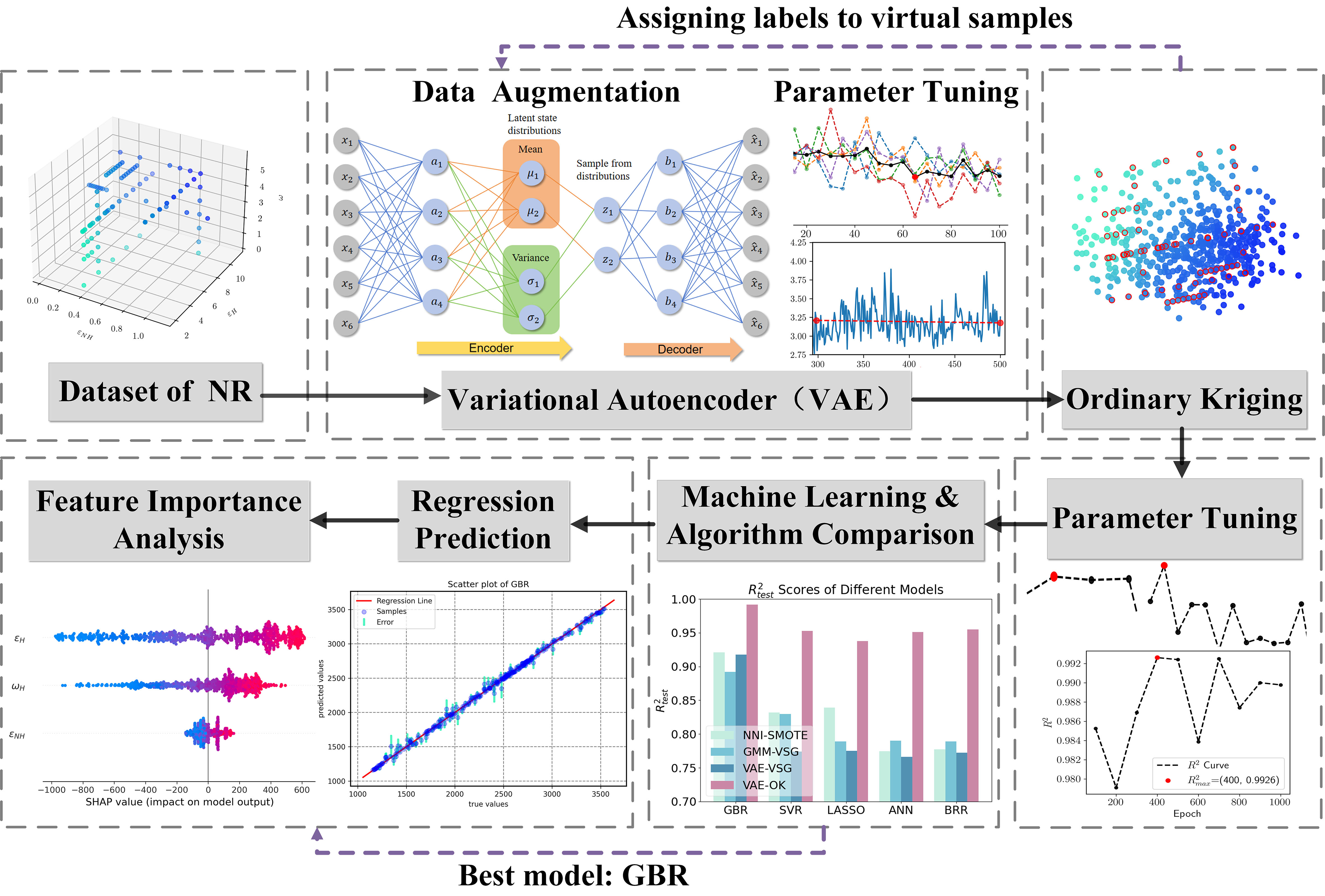
Figure 3. Flowchart of a new machine learning framework for predicting 600% tensile stress in natural rubber. NR: Natural Rubber; VAE: Variational Autoencoder; NNI-SMOTE: Nearest Neighbor Interpolation-Synthetic Minority Oversampling Technique; GMM-VSG: a Virtual Sample Generation algorithm based on Gaussian Mixture Models; VSG: Virtual Sample Generation; OK: Ordinary Kriging; GBR: Gradient Boosting Regression; SVR: Support Vector Regression; LASSO: Least Absolute Shrinkage and Selection Operator; ANN: Artificial Neural Networks; BRR: Bayesian Ridge Regression.
We have provided pseudocode in Algorithm 1 that encompasses both the VAE training and Kriging interpolation processes. This pseudocode offers a detailed description of the steps and mathematical operations involved in our methodology. We believe these additions will enhance the clarity of our approach and provide a comprehensive understanding of our new ML framework.

Algorithm 1. Algorithm VAE-OK Integration. VAE: Variational Autoencoder; OK: Ordinary Kriging.
RESULTS AND DISCUSSION
MD simulation data
In the rubber industry, tensile stress serves as a crucial parameter for evaluating the performance of rubber materials. This parameter characterizes the stress experienced by a rubber material during tensile deformation induced by an external force and is essential for conveying information about the material’s strength, ductility, and reliability. Elevated levels of tensile stress indicate that a material can withstand higher tensile forces, thus possessing greater strength. The dataset used in this study was obtained from a scholarly source, which provides detailed descriptions of the MD simulation methods and the bead-spring models for natural rubber[25]. The researchers employed MD simulation to create a coarse-grained Natural Rubber (NR) model using a bead-spring model to represent the molecular chains. The model included 100 molecular chains, each consisting of 331 beads. Additionally, the system integrates phospholipids and proteins to model the supramolecular network within natural rubber. Hydrogen bonds are established between these phospholipids or proteins and the terminal groups of the chains, including phosphate groups and polypeptides.
A total of 86 sets of NR data were derived from experimental investigations, encompassing key parameters such as the overall mass fraction of phospholipids and proteins (ω), the strength of hydrogen bonding interactions (εH), and the strength of non-hydrogen bonding interactions (εNH). These parameters are considered eigenvalues, with a tensile stress of 600% serving as the designated target value [Supplementary Materials]. Figure 4 intuitively shows the original data distribution in a 3D space and its distribution in a 2D space after dimensionality reduction by the Principal Component Analysis (PCA) algorithm. The color coding of data points corresponds to the magnitude of the 600% tensile stress.

Figure 4. Graph illustrating the distribution of data points. (A) The original data distribution in a 3D space; and (B) its distribution in a 2D space after dimensionality reduction by the PCA algorithm. PCA: Principal Component Analysis.
Data augmentation
The magnitude of data has a substantial influence on the performance of ML models. Increasing the size of the dataset enhances the model’s capability to generalize to unseen data, improves accuracy by capturing a wider range of patterns, and mitigates overfitting. Methods for augmenting data size include replicating and repeating experiments to enhance data reliability, exploring diverse samples with varying properties and preparation techniques, generating virtual data through computational simulations, and utilizing data augmentation techniques such as interpolation, extrapolation, or downsampling when there is limited availability of data.
We utilize a generative algorithm to expand the sample size by generating virtual samples from existing datasets. This approach offers several advantages, including increasing data diversity, modeling various data distributions and scenarios, and enhancing the overall applicability of the model. Additionally, it helps address data imbalances, improves model stability, and reduces the high costs associated with extensive and accurate data collection.
Generate virtual samples
The number of virtual samples generated by the VAE has a significant impact on the performance of the regression model. Insufficient virtual samples can result in underfitting and an inability to capture data patterns, while excessive virtual samples may lead to overfitting, noise problems, and reduced generalization ability of the model. Therefore, it is crucial to select an appropriate number of virtual samples. Figure 5 illustrates the distribution of virtual samples with varying numbers. The red circles represent original sample points, while the grey points indicate virtual sample points.

Figure 5. The distribution of virtual samples with varying numbers. Where red circles represent original sample points, and grey points indicate virtual sample points. (A-D) The numbers of virtual samples are 100, 300, 500, and 1000, respectively.
The number of iterations significantly influences the generation of virtual samples by VAE. Insufficient iterations may result in low quality, limited diversity, and inaccurate representation of the generated samples, while excessive iterations can lead to overfitting and resource wastage. To ensure optimal results in terms of sample quality and diversity, a balanced selection of the number of iterations should be guided by performance monitoring, early stopping strategies, and hyperparameter search. Figure 6 illustrates the distribution of virtual samples with varying numbers of iterations.

Figure 6. The distribution of virtual samples with varying numbers of iterations. Where blue circles represent original sample points, and pink points indicate virtual sample points. (A-D) The numbers of iterations are 50, 100, 300, and 500, respectively.
The VAE model can be controlled by adjusting common parameters of neural networks, such as the number of iterations, the quantity of layers in the encoder and decoder, the neuron count, and the activation function.
As shown in Figure 7A, with an increasing number of iterations, the VAE model gradually optimizes and learns the features and structure of the data, resulting in a decrease in reconstruction loss and KL divergence loss. This indicates an improvement in the model’s generation capability and the continuity of the latent space, leading to enhanced quality and diversity of generated samples. It is important to note that selecting the number of iterations is a balancing act. Too few iterations may result in the model failing to fully learn the features of the data, while too many may lead to overfitting or excessive training time. We can observe that when the number of training iterations reaches a certain threshold, the value of the loss function tends to stabilize. Although there are still some changes, they are not significant.

Figure 7. Variation of VAE loss function with iterations and neuron number. (A) Loss function values across iterations; (B) loss curves with different neuron quantities. VAE: Variational Autoencoder.
We then manipulated the number of neurons and observed their effects on the loss function value. This experiment was replicated five times, and the results are presented in Figure 7B. The curves of various colors represent multiple experiments. Despite significant fluctuations in these lines, the overall trend remained downward. The black line represents the average of these five experiments. We selected the number of neurons corresponding to the minimum loss function value on this line as the final optimal number of hidden neurons. Ultimately, we chose 65 neurons for the VAE model [Table 1].
To determine the optimal number of training iterations, we conducted multiple experiments. For different numbers of iterations, we used the VAE model to generate samples and applied the OK method to generate corresponding labels. Then, we used GBR to evaluate the quality of the generated samples using R2. We determined the optimal number of iterations by selecting the one that produced the highest-quality generated samples. Please refer to Figure 8A for specific details. We found that 400 iterations yielded the highest R2 value, indicating the best sample quality.

Figure 8. The R2 values for various parameter values within GBR model are presented. (A) The number of iterations within each epoch varies from 100 to 1,000; (B) the learning rate iterations from 0.001 to 0.01; and (C) the batch size variation from 16 to 128 iterations. GBR: Gradient Boosting Regression.
Furthermore, parameters such as the dimension of the latent variable, batch size, and learning rate can be adjusted to control the characteristics of the generated samples and ensure stability during training. Due to limitations in data dimensions, we were unable to test lower dimensions for the latent variable. Nonetheless, we can leverage the learning curve approach to optimize other critical parameters of the VAE model, thereby attaining optimal performance.
To select the optimal batch size and learning rate, we conducted multiple experiments. For each combination of batch size and learning rate, we used the VAE model to generate different samples. We then applied the OK method to generate corresponding labels and used GBR to evaluate the quality of the generated samples using the R2 metric. The batch size and learning rate that correspond to the highest R2 value are considered the best parameters. The ultimate optimal parameter combination is Learning Rate = 0.002 [Figure 8B] and Batch Size = 64 [Figure 8C], while all other parameters were kept at their default values. These parameter values yielded the maximum R2 value, indicating the highest quality of the generated samples.
Acquisition of tensile stress in virtual samples
In their study[25], to augment the dataset, the authors employed the NNI-SMOTE method. Although this approach may prove straightforward and efficient for obtaining labels of sample points, it may require smoother label values that comprehensively consider the spatial correlation of material science data. Consequently, we chose to utilize the Kriging interpolation algorithm discussed in Section “OK” to assign labels to the sample points. This algorithm effectively takes into account spatial correlation. In materials science, distributions of material properties exhibit a high degree of spatial correlation, implying that neighboring locations tend to have similar property values. Therefore, employing the Kriging interpolation algorithm provides improved rationality and interpretability when estimating property values at unmapped locations. Furthermore, Kriging interpolation can handle irregular sampling and offer reasonable estimates even at locations with missing data.
The red circle in Figure 9A delineates the distribution of the original data points. It can be observed that the newly interpolated points adhere to the distributional characteristics of the original data. Furthermore, the generated samples exhibit more continuous labels and a clearer sense of hierarchy. The two lines in Figure 9B represent kernel density estimation (KDE) curves for both labels of the original and virtual samples, respectively. Their high similarity indicates that Kriging interpolation effectively recovers the label distribution, although with some discrepancies. The differences that exist mainly at the peak of the curve are due to the fact that the distribution of virtual samples focuses more on the obvious features of the original samples, which also helps the regression model to learn from the sample data model during the training process. Moreover, the histograms in Figure 9B offer a clear comparison of the frequency distributions between the original and virtual samples. The histograms reveal that the virtual samples are well-distributed across the same range as the original samples, further confirming the effectiveness of the Kriging interpolation. The similar patterns in the histograms validate that the virtual samples accurately represent the original data, even with minor variations. By using both KDE curves and histograms, we ensure a comprehensive comparison and a deeper understanding of the data distributions.

Figure 9. (A) Scatter plot of original and virtual data points; with (B) kernel density estimation curves and histograms for their respective labels.
In addition to assessing the similarity between virtual and original samples, we have also verified the reliability of the virtual samples. Initially, we employed the Kolmogorov-Smirnov (KS) test[43] to validate the data’s accuracy. The KS test is a non-parametric statistical method used to determine whether the distributions of two independent samples are identical. The KS statistic, representing the maximum difference between the cumulative distribution functions (CDFs) of the two samples, is calculated to measure their disparity. A higher KS statistic value indicates a greater difference in distribution, with the significance of this difference assessed by the p-value. Typically, a larger p-value suggests a higher probability that the two samples follow the same distribution. We obtained the maximum, minimum, and average values of the KS statistics and p-values of the virtual and original samples from 100 repeated experiments [Table 2].
Maximum, minimum, and average values of KS Statistics and P-values for virtual and original samples from 100 repeated experiments
| KS | P-value | |
| Avg | 0.10465 | 0.44558 |
| Max | 0.132 | 0.7205 |
| Min | 0.0823 | 0.1758 |
Based on the average value, the KS statistic is small and the P-value is greater than 0.05, indicating that the distributions of the two samples are very similar. Thus, we cannot reject the hypothesis that they come from the same distribution.
Furthermore, 30 virtual samples were randomly selected from the VAE-generated data and subjected to MD simulations to validate their tensile stress at 600%. All errors were found to be below 5%, confirming the reliability of the data. To provide a clearer demonstration of this validation process and its results, we present a comparative plot of the actual data versus the VAE-generated data in Figure 10, which includes the error bounds as a shaded region, further validating the accuracy of the data. The virtual samples were sorted in ascending order of their tensile stress values, with the x-axis representing the sample index. It is important to note that the points at the same index correspond to the same characteristic, indicating that they represent the same formulation of natural rubber. The plot clearly shows that the VAE-generated data performs well within the error bounds, confirming its accuracy and reliability in simulations.

Figure 10. Comparison of MD validation and VAE-generated data for tensile stress with 5% error bounds for MD validation. MD: Molecular dynamics; VAE: Variational Autoencoder.
Comparative experiment
We conducted five sets of experiments to verify the performance of VAE-OK by comparing it with algorithms such as without virtual sample generation algorithm, NNI-SMOTE, GMM-VSG, and VAE-VSG. Here, five ML algorithms have been selected: Support Vector Regression (SVR), GBR, Least Absolute Shrinkage and Selection Operator (LASSO), Bayesian Ridge Regression (BRR), and Artificial Neural Networks (ANN). These methods are used to predictively validate the performance of the VAE-OK and assess the reasonableness of the generated virtual sample set by evaluating coefficients of determination (R2), root mean square error (RMSE), mean absolute error (MAE), and mean absolute percentage error (MAPE), which can be determined by:
Where
The first case involves no data augmentation, meaning that the raw data is used to train the prediction model. Due to the limited amount of data, we use leave-one-out cross-validation (LOOCV) method to evaluate and compare the accuracy of the model’s predictions. LOOCV is a cross-validation method that assesses the performance and generalization ability of a model by leaving only one sample point as a validation set each time while using all other samples as the training set. Since it selects differently divided datasets for each round of experiments, it can handle small sample sizes to some extent. The experiments mostly involve data-driven models, and when data is scarce, there tends to be a large gap in effectiveness among predictive models.
The experimental results are shown in Table 3. Among the models, the ANN demonstrates the worst prediction performance, and SVR also shows a poor prediction effect. Additionally, the sample is not very representative. Among them, GBR exhibits a better prediction effect; however, the highest R2 of all models is 0.8716 and the maximum MAPE is 6.49%.
Performance comparison of the five models before data augmentation
| Metrics | SVR | GBR | LASSO | ANN | BRR |
| R2 | 0.6223 | 0.8716 | 0.7681 | 0.3589 | 0.7682 |
| RMSE | 340.11 | 183.32 | 251.27 | 425.24 | 252.62 |
| MAE | 273.94 | 144.19 | 210.24 | 366.57 | 210.5 |
| MAPE | 13.22% | 6.16% | 9.22% | 30.56% | 9.22% |
Next, we utilize the sample sets generated by four virtual sample generation algorithms, namely NNI-SMOTE, GMM-VSG, VAE-VSG, and VAE-OK. Each set contains 1,000 virtual samples used for training each of the five aforementioned regression models. Figure 11 displays the R2 values of diverse models under different algorithms. When compared with other algorithms, all models trained with data generated by the VAE-OK algorithm exhibit the highest R2 values. However, there are some differences in the effectiveness of diverse models trained using samples generated by other algorithms, but they are all inferior to VAE-OK. The GBR models generally have higher R2 values compared with other algorithms, indicating their potential effectiveness in regression tasks.

Figure 11. Comparative analysis of R2 values across multiple algorithms for diverse models. NNI-SMOTE: Nearest Neighbor Interpolation-Synthetic Minority Oversampling Technique; GMM-VSG: a Virtual Sample Generation algorithm based on Gaussian Mixture Models; VAE: Variational Autoencoder; VSG: Virtual Sample Generation; OK: Ordinary Kriging; GBR: Gradient Boosting Regression; SVR: Support Vector Regression; LASSO: Least Absolute Shrinkage and Selection Operator; ANN: Artificial Neural Networks; BRR: Bayesian Ridge Regression.
Table 4 shows that all models demonstrate significantly improved prediction performance on the dataset generated by the new framework. The prediction results are highly consistent with those reported by Huang et al., but the GBR model outperforms the proposed framework in terms of prediction accuracy[25]. Furthermore, while other virtual sample generation methods fail to significantly enhance the performance of the ultimate prediction model for this dataset, VAE-OK significantly improves both the prediction accuracy and generalization capabilities of the model. Subsequently, we select the GBR with the highest performance and the ANN with the greatest performance enhancement from the prediction model, and depict the R2 values of these models as a function of the number of virtual samples in the sample set in Figure 12. In Figure 12, it is evident that models trained on virtual sample sets generated by VAE-OK algorithm outperform other data enhancement methods with similar sample sizes, demonstrating its superiority.

Figure 12. R2 value variation graph of models trained on virtual sample sets generated by multiple algorithms with varying quantities. The evaluated models are (A) the GBR, which performs the best; and (B) the ANN, which shows the highest performance improvement. NNI-SMOTE: Nearest Neighbor Interpolation-Synthetic Minority Oversampling Technique; GMM-VSG: a Virtual Sample Generation algorithm based on Gaussian Mixture Models; VAE: Variational Autoencoder; VSG: Virtual Sample Generation; OK: Ordinary Kriging; GBR: Gradient Boosting Regression; ANN: Artificial Neural Networks.
Performance comparison of the five models after data augmentation
| NNI-SMOTE | GMM-VSG | VAE-VSG | VAE-OK | ||
| GBR | R2 | 0.9439 | 0.9162 | 0.9510 | 0.9962 |
| RMSE | 153.25 | 179.02 | 119.45 | 36.69 | |
| MAE | 82.96 | 101.53 | 53.66 | 23.72 | |
| MAPE | 3.39% | 4.17% | 2.28% | 1.13% | |
| SVR | R2 | 0.8254 | 0.8294 | 0.7975 | 0.9497 |
| RMSE | 270.90 | 255.35 | 267.29 | 125.62 | |
| MAE | 197.22 | 184.10 | 186.73 | 91.27 | |
| MAPE | 7.86% | 7.69% | 7.59% | 4.59% | |
| LASSO | R2 | 0.7828 | 0.7891 | 0.7959 | 0.9419 |
| RMSE | 299.21 | 283.98 | 267.74 | 127.51 | |
| MAE | 232.74 | 214.25 | 191.90 | 97.53 | |
| MAPE | 9.87% | 9.47% | 8.58% | 4.32% | |
| ANN | R2 | 0.7719 | 0.7903 | 0.7392 | 0.9596 |
| RMSE | 306.69 | 283.12 | 261.56 | 119.09 | |
| MAE | 234.11 | 213.86 | 197.69 | 85.03 | |
| MAPE | 10.32% | 9.38% | 8.09% | 3.79% | |
| BRR | R2 | 0.7895 | 0.7893 | 0.7556 | 0.9554 |
| RMSE | 292.53 | 283.81 | 287.35 | 120.14 | |
| MAE | 224.87 | 214.04 | 229.38 | 92.04 | |
| MAPE | 9.67% | 9.46% | 9.83% | 4.14% | |
The comparison between the predictions and true values of the test set for each of the aforementioned five regression algorithms is illustrated in Figure 13. Proximity to the y = x line indicates higher accuracy in predicting sample points. The GBR model exhibits exceptional performance on the training set, with a significant number of points closely aligned with y = x. On the test set, in addition to having predictions that broadly align with experimental data, other models also demonstrate better performance on datasets generated by the new data augmentation framework, showcasing its wide applicability.

Figure 13. Visualization of the comparison and analysis between predicted values from five regression algorithms and the true values in the test set. The corresponding algorithms are as follows: (A) GBR; (B) SVR; (C) LASSO; (D) ANN; and (E) BRR. GBR: Gradient Boosting Regression; SVR: Support Vector Regression; LASSO: Least Absolute Shrinkage and Selection Operator; ANN: Artificial Neural Networks; BRR: Bayesian Ridge Regression.
Analysis of variable feature importance
To assess the individual contribution of each feature in predicting tensile stress within the GBR model, we computed the SHapley Additive exPlanations (SHAP) values for each attribute. SHAP is a specifically designed framework extensively employed in ML, including ensemble and deep learning models, for interpreting model outcomes[44]. The magnitude of SHAP values reflects the importance of each feature in the regression model. The SHAP values are determined by:
Where f(xij) is the SHAP value of xij and is the contribution vlaue of the j-th feature of xi to the predicted value yi. ybase represents the average value of the target variable across all samples.
Figure 14A illustrates the feature importance ranking, determined by averaging the absolute values of SHAP scores for each feature. Figure 14B presents the SHAP values for each molecular descriptor, with the horizontal axis representing the magnitude of influence on tensile stress prediction. Each data point corresponds to a sample, with GBR predicting its output value. The color of points in the chart transitions to redder hues as feature values increase. It is evident that all variables are positively correlated with the tensile stress of NR. The obtained results lead us to a plausible conclusion that εH exerts the primary influence on the NR’s tensile stress, followed by ω and ultimately εNH.

Figure 14. Analysis of feature importance for each feature descriptor. (A) The bar chart summarizes the feature importance, with features ordered based on the average absolute value of SHAP; (B) the density scatter plot also summarizes the feature importance. SHAP: SHapley Additive exPlanations.
In natural rubber, molecules typically maintain their structure through hydrogen bond interactions. These relatively strong intermolecular forces can significantly influence the mechanical properties of materials. Consequently, the strength of hydrogen bond interactions has a substantial impact on tensile stress. The presence of impurities such as phospholipids and proteins in natural rubber can alter its structure and performance by interacting with rubber molecules, leading to changes in molecular structure and aggregation that ultimately affect the elasticity and tensile strength of rubber. In contrast, non-hydrogen bond interactions are typically weaker intermolecular forces that may not have enough potency to significantly influence the mechanical properties of natural rubber. Hence, the strength of non-hydrogen bond interactions has a relatively minor effect on tensile stress. This may be attributed to the significant strength of hydrogen bond interactions, which play a dominant role in tensile stress. These hydrogen bonds tend to create stronger affinities between rubber molecules, thus influencing the material’s tensile performance.
CONCLUSIONS
This work presents a new algorithm for generating virtual samples based on the VAE framework. The main innovation lies in applying pre-interpolation techniques to stabilize the distribution of the initial dataset, resulting in virtual samples that exhibit a higher degree of conformity with the original data distribution. In the process of computing labels, we employ the OK method, making full use of the labels in the original dataset, ensuring that the labels of virtual samples better align with the spatial characteristics of materials science data.
We validate the effectiveness of the proposed VAE-OK method using a small dataset of natural rubber material. Experimental findings suggest that VAE-OK effectively infers and expands the initial training dataset, resulting in a significant improvement in model accuracy ranging from 13% to 160%, compared to scenarios without sample extension. Compared to conventional interpolation-based virtual sample generation methods, the VAE-OK outperforms numerous ML models.
The VAE-OK algorithm not only enhances the accuracy of small-sample ML models but also demonstrates its versatility by reducing the need for repetitive chemical experiments and physical calculations. Furthermore, this new approach provides invaluable insights into the discovery and analysis of factors that influence the tensile stress of natural rubber polymers. Guided by this research methodology and its findings, predicting tensile stress in natural rubber becomes more precise while simultaneously expanding possibilities for predicting other material properties or performance with limited data.
Looking forward, an important avenue for future research will be to extend the VAE-OK framework to accommodate multi-axial loading conditions. Incorporating multi-axial stress data into the model and adapting the simulation setup to manage simultaneous stresses in multiple directions represents a significant research opportunity. This development will be crucial for enhancing the comprehensiveness of our predictive framework and its applicability to a broader range of real-world scenarios. We believe that exploring this direction will significantly advance our understanding of material behavior under complex loading conditions.
DECLARATIONS
Authors’ contributions
Conceptualization, methodology, writing - original draft preparation, software: Hu A, Liu Z
Formal analysis: Hu A, Chen Q
Investigation, data curation: Chen Q, Zhan S, Li Q
Writing - review and editing: Hu A, Liu Z, Zhan S
Supervision: Cui L, Liu J
Availability of data and materials
The data and source code that support the findings of this study are available from the corresponding author upon reasonable request.
Financial support and sponsorship
This work was supported by the National Science Fund for Excellent Young Scholars (52122311) and the National Natural Science Foundation of China (52373222, 92367111).
Conflicts of interest
Liu J is Junior Editorial Board Member of the Journal of Materials Informatics, while the other authors have declared that they have no conflicts of interest.
Ethical approval and consent to participate
Not applicable.
Consent for publication
Not applicable.
Copyright
© The Author(s) 2024.
Supplementary Materials
REFERENCES
1. Chibani S, Coudert FX. Machine learning approaches for the prediction of materials properties. APL Mater 2020;8:080701.
2. Li D, Ru Y, Chen Z, Dong C, Dong Y, Liu J. Accelerating the design and development of polymeric materials via deep learning: current status and future challenges. APL Mach Learn 2023;1:021501.
3. Geng X, Wang F, Wu HH, et al. Data-driven and artificial intelligence accelerated steel material research and intelligent manufacturing technology. Mater Genome Eng Adv 2023;1:e10.
4. Shi R, Wang X, Song X, et al. Tensile performance and viscoelastic properties of rubber nanocomposites filled with silica nanoparticles: a molecular dynamics simulation study. Chem Eng Sci 2023;267:118318.
5. Yagyu H. Coarse-grained molecular dynamics simulation of the effects of strain rate on tensile stress of cross-linked rubber. Soft Mater 2015;13:263-70.
6. Frankland SJV, Harik VM, Odegard GM, Brenner DW, Gates TS. The stress-strain behavior of polymer-nanotube composites from molecular dynamics simulation. Compos Sci Technol 2003;63:1655-61.
7. Odegard GM, Jensen BD, Gowtham S, Wu J, He J, Zhang Z. Predicting mechanical response of crosslinked epoxy using ReaxFF. Chem Phys Lett 2014;591:175-8.
8. Chung I, Im S, Cho M. A neural network constitutive model for hyperelasticity based on molecular dynamics simulations. Numer Meth Eng 2021;122:5-24.
9. Lee J, Wang H, Kim JH, Shin H. Importance of cohesive failure mode in fracture toughness enhancement of polymer nanocomposites with covalent grafting: a multiscale study. Compos Part B Eng 2024;279:111462.
10. Wang H, Lee J, Kim JH, Shin H. Multiscale strategy to predict the fracture toughness and crack extension behavior of ozone-functionalized carbon nanotube/epoxy nanocomposites. Chem Eng J 2023;465:142985.
11. Chen Q, Huang W, Duan P, et al. Manipulating the mechanical properties of cis-polyisoprene nanocomposites via molecular dynamics simulation. Polymer 2022;256:125233.
12. Chen Q, Zhang Z, Huang Y, et al. Structure-mechanics relation of natural rubber: insights from molecular dynamics simulations. ACS Appl Polym Mater 2022;4:3575-86.
13. Le Cam JB, Huneau B, Verron E, Gornet L. Mechanism of fatigue crack growth in carbon black filled natural rubber. Macromolecules 2004;37:5011-7.
14. Trabelsi S, Albouy P, Rault J. Stress-induced crystallization around a crack tip in natural rubber. Macromolecules 2002;35:10054-61.
15. Shen L, Qian Q. A virtual sample generation algorithm supporting machine learning with a small-sample dataset: a case study for rubber materials. Comput Mater Sci 2022;211:111475.
16. Lockner Y, Hopmann C, Zhao W. Transfer learning with artificial neural networks between injection molding processes and different polymer materials. J Manuf Process 2022;73:395-408.
17. Chen Z, Li D, Liu J, Gao K. Application of Gaussian processes and transfer learning to prediction and analysis of polymer properties. Comput Mater Sci 2023;216:111859.
18. Kim Y, Kim Y, Yang C, Park K, Gu GX, Ryu S. Deep learning framework for material design space exploration using active transfer learning and data augmentation. npj Comput Mater 2021;7:609.
19. Akdemir A. Research on task discovery for transfer learning in deep neural networks. In: Proceedings of the 58th Annual Meeting of the Association for Computational Linguistics: Student Research Workshop. Association for Computational Linguistics; 2020. pp. 33-41.
20. Wu X, Manton JH, Aickelin U, Zhu J. A Bayesian approach to (online) transfer learning: theory and algorithms. Artif Intell 2023;324:103991.
21. Zhang Y, Fang Y, Li L, et al. Thermal stability prediction of copolymerized polyimides via an interpretable transfer learning model. J Mater Inf 2024;4:8.
22. Xu P, Ji X, Li M, Lu W. Virtual sample generation in machine learning assisted materials design and discovery. J Mater Inf 2023;3:16.
23. Li D, Liu J, Liu J. NNI-SMOTE-XGBoost: A novel small sample analysis method for properties prediction of polymer materials. Macromol Theory Simul 2021;30:2100010.
24. Hu A, Huang Y, Chen Q, et al. Glass transition of amorphous polymeric materials informed by machine learning. APL Mach Learn 2023;1:026111.
25. Huang Y, Chen Q, Zhang Z, et al. A machine learning framework to predict the tensile stress of natural rubber: based on molecular dynamics simulation data. Polymers 2022;14:1897.
26. Radford A, Metz L, Chintala S. Unsupervised representation learning with deep convolutional generative adversarial networks. arXiv. [Preprint.] Jan 7, 2016 [accessed 2024 Aug 14]. Available from: https://arxiv.org/abs/1511.06434.
27. Nguyen A, Dosovitskiy A, Yosinski J, Brox T, Clune J. Synthesizing the preferred inputs for neurons in neural networks via deep generator networks. In: NIPS’16: Proceedings of the 30th International Conference on Neural Information Processing Systems. Curran Associates Inc.; 2016. pp. 3395-403. Available from: https://dl.acm.org/doi/abs/10.5555/3157382.3157477. [Last accessed on 14 Aug 2024]
28. Zhu JY, Krähenbühl P, Shechtman E, Efros AA. Generative visual manipulation on the natural image manifold. arXiv. [Preprint.] Dec 16, 2018 [accessed 2024 Aug 14]. Available from: https://arxiv.org/abs/1609.03552.
29. Denton E, Chintala S, Szlam A, Fergus R. Deep generative image models using a Laplacian pyramid of adversarial networks. In: Proceedings of the 28th International Conference on Neural Information Processing Systems - Volume 1. Cambridge, MA, USA: MIT Press; 2015. pp. 1486-94. Available from: https://dl.acm.org/doi/10.5555/2969239.2969405. [Last accessed on 14 Aug 2024]
30. Chen Q, Liu Z, Huang Y, et al. Predicting natural rubber crystallinity by a novel machine learning algorithm based on molecular dynamics simulation data. Langmuir 2023;39:17088-99.
31. Arjovsky M, Bottou L. Towards principled methods for training generative adversarial networks. arXiv. [Preprint.] Jan 17, 2017 [accessed 2024 Aug 14]. Available from: https://arxiv.org/abs/1701.04862.
32. Kingma DP, Welling M. Auto-encoding variational bayes. arXiv. [Preprint.] Dec 10, 2022 [accessed 2024 Aug 14]. Available from: https://arxiv.org/abs/1312.6114.
33. Kulkarni TD, Whitney WF, Kohli P, Tenenbaum JB. Deep convolutional inverse graphics network. arXiv. [Preprint.] Jun 22, 2015 [accessed 2024 Aug 17]. Available from: https://arxiv.org/abs/1503.03167.
34. Gregor K, Danihelka I, Graves A, Rezende DJ, Wierstra D. DRAW: a recurrent neural network for image generation. arXiv. [Preprint.] May 20, 2015 [accessed 2024 Aug 14]. Available from: https://arxiv.org/abs/1502.04623.
35. Sønderby CK, Raiko T, Maaløe L, Sønderby SK, Winther O. Ladder variational autoencoders. In: NIPS’16: Proceedings of the 30th International Conference on Neural Information Processing Systems. Red Hook, NY, USA: Curran Associates Inc.; 2016. pp. 3745-53. Available from: https://dl.acm.org/doi/abs/10.5555/3157382.3157516. [Last accessed on 14 Aug 2024]
36. Im DI, Ahn S, Memisevic R, Bengio Y. Denoising criterion for variational auto-encoding framework. AAAI 2017;31:1.
37. Wang X, Liu H. Data supplement for a soft sensor using a new generative model based on a variational autoencoder and Wasserstein GAN. J Process Control 2020;85:91-9.
38. Ohno H. Auto-encoder-based generative models for data augmentation on regression problems. Soft Comput 2020;24:7999-8009.
39. Kulosa M, Neumann M, Boeff M, Gaiselmann G, Schmidt V, Hartmaier A. A study on microstructural parameters for the characterization of granular porous ceramics using a combination of stochastic and mechanical modeling. Int J Appl Mechan 2017;09:1750069.
40. Díaz-montiel P, Escalona-galvis L, Venkataraman S. Kriging and dimension reduction techniques for delamination detection in composites using electrical resistance tomography. Eng Optim 2023;55:19-34.
41. Kookalani S, Cheng B, Torres JLC. Structural performance assessment of GFRP elastic gridshells by machine learning interpretability methods. Front Struct Civ Eng 2022;16:1249-66.
42. Daya AA, Bejari H. A comparative study between simple kriging and ordinary kriging for estimating and modeling the Cu concentration in Chehlkureh deposit, SE Iran. Arab J Geosci 2015;8:6003-20.
44. Lundberg S, Lee SI. A unified approach to interpreting model predictions. arXiv. [Preprint.] Nov 25, 2017 [accessed 2024 Aug 14]. Available from: https://arxiv.org/abs/1705.07874.
Cite This Article

How to Cite
Download Citation
Export Citation File:
Type of Import
Tips on Downloading Citation
Citation Manager File Format
Type of Import
Direct Import: When the Direct Import option is selected (the default state), a dialogue box will give you the option to Save or Open the downloaded citation data. Choosing Open will either launch your citation manager or give you a choice of applications with which to use the metadata. The Save option saves the file locally for later use.
Indirect Import: When the Indirect Import option is selected, the metadata is displayed and may be copied and pasted as needed.
About This Article
Special Topic
Copyright


Comments
Comments must be written in English. Spam, offensive content, impersonation, and private information will not be permitted. If any comment is reported and identified as inappropriate content by OAE staff, the comment will be removed without notice. If you have any queries or need any help, please contact us at [email protected].