


DSMR: an AI framework for exploring combinations of data and algorithm to overcome efficiency-accuracy trade-off
 0
0 Abstract
Machine learning models demonstrate remarkable capabilities in predicting properties of novel material. The optimal model can theoretically be obtained through an exhaustive search of data subsets, algorithms, and hyperparameters. However, the fundamental challenge lies in identifying the most efficient pathway through this immense search space. In this paper, we address this challenge by proposing an active learning-based data screening and model retrieval framework, which can develop enhanced models based on internal data while incorporating additional external data to further improve model performance. Systematic validation studies were conducted using four datasets, comprising both classification and regression data. Superior models were obtained within 10 iterative cycles for all cases, achieving a 3.3%-10.3% improvement compared to state-of-the-art results in current literature. Among the results, the framework reduced modeling error by 10.3% for AlCoCrCuFeNi hardness internal data and achieved a more significant error reduction of 42.6% through the integration of additional external hardness data. The framework achieves an ideal balance between computational efficiency and predictive accuracy while enabling deeper data exploration, with its low-code implementation and user-friendly characteristics making it a promising tool for materials design.

Keywords
INTRODUCTION
A data-driven approach has the potential to significantly reduce the cost and time associated with materials development processes[1-3]. Researchers can use machine learning models to predict the properties of novel materials and identify trends, even in the absence of a full understanding of the underlying physical mechanisms[4,5].
However, most existing studies merely generate locally optimal models based on limited data and specific algorithms, failing to fully exploit the dataset’s information. For example, Wen et al. found that the support vector regression (SVR)-radial basis function (rbf) model was best suited to the AlCoCrCuFeNi hardness dataset, achieving a root mean square error (RMSE) of 68 HV, which was subsequently used as a baseline model for active learning[6]. Building upon this work, Li et al. enhanced the dataset, resulting in a reduced RMSE of 53 HV for the SVR-rbf model[7]. Furthermore, Zhang et al. demonstrated that a stacking algorithm based on a combination of CatBoost and LightGBM outperformed the SVR model when evaluated on the expanded dataset[8]. Overall, even with the same system, changing the combinations of data and algorithms may lead to different results. In theory, exploring the combinations of data subsets, algorithms, and hyperparameters can yield the optimal model.
Datasets are typically represented in matrix form, where rows represent samples and columns stand for features. The selection of both samples and features determines the final model’s performance. Feature selection methods are well-established, such as tree-based importance analysis[9], which assesses a feature’s contribution to model performance by its impact on split nodes; recursive feature elimination (RFE) repeatedly trains a model[10], gradually removing the redundancy features based on model performance or feature importance, until an optimal subset is left; principal component analysis (PCA) reduces high-dimensional feature set by mapping it to fewer principal components while preserving the most important information[11,12]. In addition, some researchers have integrated common methods. For instance, Zhang et al. combined correlation screening, recursive elimination, and exhaustive search to extract key features for copper alloys, establishing a new Hall-Petch relationship[13,14]. However, sample selection is more complex and tedious. It requires not only collecting representative samples to maintain their distribution in high-dimensional space but also carefully filtering noise to preserve model robustness. Unlike feature selection, which directly provides feature importance, the importance of individual samples emerges through a “contextual” effect in combination with other samples.
The mainstream of existing research methods for sample optimization contains noisy sample filtering, unbalanced data processing and active learning data sampling. Noisy sample filtering works by identifying and removing samples in the dataset that are clearly anomalous or mislabeled, but may mistakenly remove samples that do not fit the regular pattern but are critical to model learning[15]. Unbalanced data processing can address the dominance of majority class samples and improve the prediction performance of minority class samples. However, it may lead to issues such as excessive oversampling repetition or insufficient data quantity in undersampling[16]. Active learning data sampling selects the most representative subset of samples from the entire dataset based on their contribution to model training. Li et al. used an uncertainty-based active learning approach to reduce redundancy in several authoritative large datasets, creating a smaller yet equally informative dataset[17]; Chen et al. developed the active learning-based data screening (ALDS) framework based on active learning, utilizing a high-quality internal small dataset to filter multi-source external data and expand the small dataset into a larger one[18]. However, current research approaches overlook two critical issues. First, methods that rely exclusively on elimination fail to consider the potential “contextual” relationships between external samples and the internal dataset, while addition-only strategies cannot effectively evaluate the distribution quality of existing internal samples. Second, the practice of data evaluation using limited algorithmic approaches fails to address the varying effectiveness of different algorithms across diverse scenarios.
This paper proposes a data screening (DS) and model retrieval (MR) framework based on active learning (DSMR), distinguished by its integration of sample optimization through elimination/addition and standardized MR methods, aimed at recommending the most suitable data and algorithm for designers. The DS methods in the DSMR framework are based on a “leave-one-out” approach for gradual elimination and addition, incorporating the concept of cross-validation to maintain the original data distribution. The MR methods also integrate most mainstream regression and classification machine learning algorithms, utilizing Bayesian optimization to effectively explore potential combinations of algorithms and hyperparameters, while employing common evaluation metrics to assist in model exploration. The effectiveness and robustness of DSMR in DS and MR have been validated across various classification and regression datasets, including perovskites, steel, and high-entropy alloys (HEAs). The DSMR framework can develop enhanced models based on internal data while incorporating additional external data to further improve model performance.
MATERIALS AND METHODS
Overview and architecture
The primary goal of DSMR is to assess the importance of each row in the data matrix (i.e., each sample) and provide materials scientists with the optimal combination of data subsets and models. To train predictive models on DSMR, users need to upload a CSV file containing the feature matrix X and the target variable Y. The feature matrix X includes material compositions and processing information, while the target variable Y contains one or more material properties, with each sample corresponding to its respective X and Y. As shown in Figure 1, the DS module achieves data enhancement through a “leave-one-out” approach for data elimination and addition, preserving the original sample distribution during the elimination process and recovering valid samples during the addition process. The MR module is based on generic algorithm integration and Bayesian autotuning for optimal model selection, enabling comprehensive evaluation of algorithmic suitability while maintaining standardized hyperparameter optimization. This module supports nearly all widely used algorithms, such as linear model, support vector machine, random forest, and XGBoost, each with its own advantages, ensuring comprehensive data evaluation. The MR module incorporates Bayesian hyperparameter optimization, using surrogate models in conjunction with acquisition functions to select the best hyperparameters. This approach accelerates the global optimization of model parameters while minimizing human intervention[19,20]. Additionally, the evaluation metrics for MR are based on the RMSE and R2 for regression models, along with Accuracy for classification models, ensuring fairness and min-max normalization in the evaluation.

Figure 1. Overview and architecture of DSMR. (A) The DS module employs a “leave-one-out” approach for gradual elimination and addition, extracting key data samples while preserving the overall data distribution; (B) The MR module integrates algorithm ensemble, automatic parameter tuning, and evaluation ranking, providing a unified modeling and evaluation process to ensure comprehensive and fair assessment of data subsets. DSMR: Data screening and model retrieval framework based on active learning.
The two modules of the DSMR framework work together during the iteration process, continuously recombining data and exploring models, and finally determining whether to continue iteration based on evaluation metrics. In this process, the DS module only provides possible data combinations, while the MR module is responsible for standardized machine learning modeling. The detailed hyperparameter adjustment range of the DSMR framework is shown in Supplementary Table 1.
As shown in Figure 2, the DSMR framework explores the three-dimensional space of optimal data subsets, algorithms, and hyperparameters. The MR module of the framework acts similar to a child seeking a path, exploring the three-dimensional space to find the optimal combination. Guided by Bayesian optimization, the child possesses the ability for global exploration. Meanwhile, evaluation metrics act as a compass, guiding the gradual optimization of the model, while the DS module adjusts the data to provide the child with suitable learning materials. During the iterative process, the dataset (X, Y) first undergoes a round of random shuffling, followed by step Figure 2A, where it is divided into subsets of size N, with each subset eliminating a different portion to prevent excessive differences in data distribution. Next, each subset enters the MR module in step Figure 2B, where normalization is applied, and Bayesian optimization is used to globally explore the hyperparameter combinations of the chosen algorithms. Then, step Figure 2C employs cross-validation to evaluate the results, ranking all models by performance, retaining the best model and data subset combination, and selecting the optimal subset K for the next round. If data elimination reaches a performance bottleneck, the framework switches to step Figure 2D to recycle samples, similarly dividing and re-adding the eliminated data by size N, and entering the MR module for model exploration. Finally, step Figure 2E continues to evaluate and rank the models, terminating the process when model performance reaches a bottleneck or data can no longer be divided.

Figure 2. Flowcharts of subset selection and model construction in DSMR. (A) Subset partitioning rules for data elimination; (B) The MR module retrieves in the three-dimensional space of data subsets, algorithms, and hyperparameters using Bayesian optimization and standardized evaluation; (C) Data elimination subset ranking and iterative assessment; (D) Subset partitioning rules for data addition; (E) Data addition subset ranking and iterative assessment. DSMR: Data screening and model retrieval framework based on active learning.
DSMR provides a comprehensive workflow for data sampling and MR, as shown in Figure 2. The abbreviations of the specific machine learning methods and materials systems used are shown in Table 1. Implementing the full DSMR process requires attention to several details in data processing and model construction, including data normalization, Bayesian optimization, cross-validation evaluation, and the core “leave-one-out” strategy for the gradual elimination and addition of data.
Abbreviations of machine learning methods and materials systems
| Nomenclature | |||
| LR[21] | Logic regression | SVR[21] | Support vector regression |
| XGBR[22] | XGBoost regression | ETR[21] | Extra trees regression |
| MLPR[21] | Multi-layer perception regression | KNNR[21] | K-nearest neighbor regression |
| RFR[21] | Random forest regression | CBR[23] | CatBoost regression |
| SVC[21] | Support vector classification | DTC[21] | Decision tree classification |
| RFC[21] | Random forest classification | XGBC[22] | XGBoost classification |
| CBC[23] | Gradient boosting classification | BTC[21] | Bagging tree classification |
| R2 | Determination coefficient | RMSE | Root mean squared error |
| LOO | Leave one out | HV | Vickers hardness |
| TE | Total elongation | PCF | Polycrystalline ceramic formability |
Data preparation
This study employs min-max normalization as a data processing method. As given in
Here, x represents a single feature. This approach involves iterating through each column of the input features to record the maximum and minimum values, then scaling the data to a range of 0 to 1 using a specific formula. Normalizing the data aims to accelerate the speed of gradient descent during the training process while potentially improving accuracy, all without disrupting the underlying distribution of the original data[24]. In machine learning or deep learning, most models’ loss calculations assume that all features have a mean of zero and the same variance. This uniformity allows for consistent processing of all feature attributes during loss computation. If two sample attributes have significantly different scales, the attribute with the larger scale can dominate the distance calculations, which may not reflect the true relationships in the data. To address this issue, min-max normalization is applied to scale the feature attributes to a common dimension, helping to mitigate the impact of scale differences.
Machine learning method
Leave-one-out cross-validation (LOO) and K-fold cross-validation are widely used for model validation[25,26]. The core mechanism of LOO involves removing one data point at a time, using the remaining N - 1 points as the training set and the removed point as the validation set. For a dataset with N points, LOO repeats this process N times, each time with a different point as the validation set. This method decreases the training set size by one point in each iteration while incrementally increasing the validated data points back into the training set. The training set for each round can be expressed as D - Di and the validation set as Di, iterating over all i ∈ [1, N]. LOO’s strength lies in utilizing all available data for validation; however, because it only removes one point at a time, its computational cost is O(N2), making it expensive for large datasets. K-fold cross-validation, on the other hand, works by dividing the dataset into K subsets. Each time, K - 1 subsets are used as the training set and the remaining one as the validation set. This process is repeated K times, with each subset being used as the validation set at least once. The training set can be denoted as Dtrain = D - Di and the validation set as Di, with the final validation error averaged across all rounds. The rationale behind K-fold is that by partitioning the data, it reduces both variance and bias while ensuring that each sample is used for both training and validation. Its time complexity is O(N), providing higher computational efficiency for medium to small-sized datasets.
In regression tasks, the coefficient of determination (R2) and the RMSE are key indicators of model performance. R2 measures the model’s ability to explain the variance in the data, with values closer to 1 indicating better fit. RMSE quantifies the average error between predicted and actual values. In classification tasks, accuracy reflects the overall predictive performance of the classifier across all samples.
Here, y represents the observed values, y denotes the predicted values, and n is the number of samples. TP and TN refer to the true positives and true negatives, respectively, while FP and FN indicate the false positives and false negatives.
Bayesian hyperparameter optimization is introduced, whereby the ability to select the best hyperparameters is provided using a surrogate model combined with an acquisition function. The pseudo-code of Bayesian hyperparameters optimization is provided in Table 2.
Bayesian hyperparameter optimization pseudo-code
| Algorithm 1 Sequential Model-Based Optimization |
| Input: f, for i ← | p(y|x, xi ← arg yi ← f(xi) end for |
where f stands for the hyperparameter-loss function relationship,
RESULTS AND DISCUSSION
Regression verification
Hardness prediction of HEAs
The hardness data of cast HEAs is often used in conjunction with machine learning methods to recommend high-hardness compositions, as it is less influenced by processing conditions and is easy to validate[7,8,27,28]. In 2019, Wen et al. obtained the best baseline model SVR-rbf with an RMSE error of 68 HV by manually tuning parameters based on 155 sets of AlCoCrCuFeNi hardness data and 8 algorithms[6]. Supplementary Table 2 shows the basics of the Wen’s data, with features consisting only of components, modeled with Vickers hardness as the target value.
In this paper, the same dataset (designated as Wen-HV) was integrated with the regression algorithm in the DSMR framework, through which an optimized data-algorithm combination was obtained, yielding a cross-validation RMSE of 61 HV and reducing the error by 10.3%. The model’s generalization capability was validated using an independent test set, achieving an RMSE of 61 HV. Figure 3A illustrates the processing and evaluation of data subsets in the DSMR framework. The blue background represents data elimination, with a step size N of 10, constructing 10 different data subsets by eliminating 10% in each round. The white dots represent models customized by the MR module for each data subset, while the red indicates the best combination for that round, corresponding to the optimal subset K for the next iteration. In the second iteration, a cross-validation combination achieves an RMSE of 60 HV. After continuing the elimination, the error increases, prompting a transition to the orange background addition phase, where some potentially critical samples are re-added to the dataset for evaluation. However, the error still rises after re-addition, leading to process termination. Comparison of all combinations shows that the mean error remains nearly constant in each iteration; however, the results from the second iteration indicate that slight differences in data can lead to significant performance variations in models. Figure 3B presents the RMSE errors for the best models from six algorithms on the validation set (20%) and an independent test set (5%) during the second iteration. Under the same algorithmic conditions, the SVR model optimized by the DSMR framework has an RMSE of 52 HV on the validation set, outperforming the SVR-rbf baseline model constructed by Wen, but demonstrating weaker generalization with an RMSE of only 78 HV on the independent test set. In contrast, the ETR model performs excellently on both the validation and independent test sets. Thus, Figure 3C shows a comparison of true and predicted values for the ETR model on the training and validation sets, with points in the training set closely aligned along the perfect fit line and a validation RMSE of 60 HV. To further validate the model’s generalization capability, we randomly select 5% of the data as a test set for validation in Figure 3D, ensuring the test set is not involved in training or model tuning. The results indicate that the ETR model maintains high predictive capability on unknown data, achieving an RMSE of 61 HV. Overall, the ETR model outperforms the Wen-optimized baseline model on both the validation and independent test sets.

Figure 3. Data sampling and model construction for the Wen-HV dataset. (A) Exploration of Wen-HV data subsets and algorithm combinations, along with the performance of the original baseline model. The white dots denote the performance of each data subset-algorithm pairing, whereas the red dot highlights the optimal combination achieved in this iteration. The black, blue, and red lines represent the article’s baseline model’s 10-fold accuracy, the data elimination process, and the data addition process, respectively; (B) Error performance of six algorithms on the validation and test sets; (C) Comparison of true and predicted values for the best generalization model, ETR, on the training and test sets; (D) Comparison of true and predicted values for the ETR model on the test set. ETR: Extra trees regression.
Total elongation predicted for reduced activation ferritic-martensitic
Reduced activation ferritic-martensitic (RAFM) steel has been developed from conventional 9Cr-1Mo steel and is considered a promising structural material candidate for fusion reactors due to its excellent thermophysical, thermomechanical, and radiation resistance, especially compared to austenitic steels[29,30]. In 2024, Ma et al. utilized 274 RAFM steel total elongation (TE) data points, over 11 regression algorithms from the MLMD regression module, and the NSGA-II algorithm from the surrogate optimization module to design RAFM steel with high strength and excellent ductility[28]. The best baseline model achieved a cross-validation R2 of only 0.7760. Supplementary Table 3 shows the basic situation of Ma’s data; the characteristics include basic conditions such as composition and temperature, and the TE is modeled as the target value.
In this paper, the same dataset (designated as Ma-TE) was integrated with regression algorithms from the DSMR framework, through which an optimized data-algorithm combination was achieved, yielding a cross-validation R2 of 0.8270 and improving accuracy by 6.6%. The model’s generalization capability was subsequently validated using an independent test set, achieving an R2 of 0.8843. Figure 4A illustrates the processing and evaluation of data subsets by the DSMR framework. The blue background indicates the data splitting section, with a step size N of 10, where 10 different data subsets are constructed by eliminating 10% in each round. The white dots represent models customized by the MR module for each data subset, while the red dot indicates the combination with the highest R2 for that round, corresponding to the best subset K for the next iteration. In the fourth iteration, a combination was found that achieved a cross-validation R2 of 0.8270. However, further elimination in the blue background or addition in the orange background did not lead to performance improvements, resulting in process termination. Comparing all combinations shows that the average accuracy increases with each iteration, indicating improved model quality. Then, after two attempts at data addition, the accuracy of the combinations did not significantly rise, suggesting a lack of effective data that connects the retained samples with those removed. Figure 4B presents the R2 for six algorithms, showcasing the best model from the second iteration on a validation set (20%) and an independent test set (5%). Since Ma-TE did not specify the algorithm used for its baseline model, a direct comparison under the same conditions was not possible. Nevertheless, the XGBR model optimized by the DSMR framework achieved an R2 of 0.9412 on the validation set and 0.8843 on the test set, significantly outperforming the Ma-TE baseline model’s R2 of 0.7760. Figure 4C compares the true and predicted values for the training and validation sets of the XGBR model, showing that the adjusted model effectively learns the data patterns in the training set, with points mostly falling on the perfect fit line. The R2 for the validation set reached 0.9412, with an RMSE of 1.55%. To further validate the model’s generalization capability, we randomly selected 5% of the data as a test set, which was not involved in training. Figure 4D compares the true and predicted values of the XGBR model on the test set, achieving an R2 of 0.8843, indicating high predictive power in unknown data. It can be concluded that the Ma-TE baseline model has undergone meticulous optimization, suggesting that without changing the data, the optimization limit is the performance level reached by the MLMD framework. However, through DSMR’s DS and MR, it is possible to efficiently obtain models with superior performance, and this process is not limited to mere model adjustments.

Figure 4. Data sampling and model construction for the Ma-TE dataset. (A) Exploration of MLMD-TE data subsets and algorithm combinations, including the original baseline model’s 10-fold R2 value; (B) Presentation of error performance for six algorithms on the validation and test sets; (C) Comparison of true and predicted values for the best generalization model XGBR on the training and validation sets; (D) Comparison of true and predicted values for the XGBR model on the test set. R2: Determination coefficient; XGBR: XGBoost regression.
Classification verification
Binary classification prediction of formability in polycrystalline ferroelectric ceramics
Polycrystalline ferroelectric ceramics are important materials widely used in sensors, actuators, and storage devices, with their crystal structure significantly influencing ferroelectric properties[31]. These ceramics can be broadly classified into two categories: perovskite and non-perovskite structures. Perovskite materials typically exhibit high dielectric constants and excellent ferroelectric performance, making them highly valuable in electronic devices[32,33]. In 2024, Ma et al. used 192 sets of polycrystalline ceramic moldability data combined with 6 algorithms in the MLMD classification module to design a classification model for distinguishing polycrystalline ferroelectric ceramic structures[28]. After MLMD optimization, the best baseline model achieved a cross-validation accuracy of 0.8650. Supplementary Table 4 shows the basics of Ma’s data, characterized by elements’ physicochemical properties such as tolerance factor, modeled with formability as the target value.
In this paper, the same dataset (designated as Ma-PCF) was integrated with classification algorithms in the DSMR framework, through which an optimized data-algorithm combination was achieved, yielding a cross-validation R2 of 0.9490 and improving accuracy by 9.7%. The model’s generalization capability was subsequently validated using an independent test set, from which an R2 of 0.8000 was obtained. Figure 5A shows the processing and evaluation of data subsets in the DSMR framework. The blue background indicates the data partitioning section, with a step size of N equal to 10, and each round removing 10% to create 10 different subsets. The white dots represent the models customized for each data subset by the MR module, while the red indicates the highest Accuracy combination for that round, corresponding to the best subset K for the next iteration. In the sixth round, a cross-validation Accuracy of 0.9490 was achieved. Subsequent iterations showed no further performance improvements in either the blue background (elimination) or orange background (addition) regions, leading to process termination. Comparisons show that nearly all new models explored by DSMR have cross-validation Accuracy exceeding that of the Ma-PCF models, suggesting that model performance may depend more on data sampling than on hyperparameter optimization, given the same feature selection. Figure 5B illustrates the Accuracy for the best models from six algorithms during the second iteration, evaluated on the validation set (20%) and an independent test set (5%). In terms of model consistency with the Ma-PCF models, we replaced BTC with DTC, as RFC extends BTC by increasing feature randomness, thereby enhancing model robustness and generalization while reducing overfitting. Although DTC is a single tree model prone to overfitting, it offers strong interpretability. In terms of performance, DTC, RFC, XGBC, and CBC models outperformed the Ma-PCF baseline model on the validation set, with CBC achieving 100% accuracy on both training and test sets. However, performance on the independent test set was relatively poor, likely due to the limited size of the randomly selected validation set (only 10 data points), significantly impacting results. Figure 5C presents the confusion matrix for the best CBC model across the training, validation, and test sets, showing a complete match between predicted and actual classifications. Despite the relatively unbalanced distribution of perovskite and non-perovskite structures, the validation set achieved 100% Accuracy, surpassing the Ma-PCF baseline of 0.8650. To further validate generalization, we randomly selected 5% of the data as an independent test set not involved in training; the confusion matrix indicates the model maintains 80% accuracy on unseen data. Figure 5D depicts the ROC curve for the CBC model, illustrating the relationship between true positive rate (TPR) and false positive rate (FPR). TPR indicates sensitivity, while FPR is calculated as 1 minus specificity. The curve is plotted with FPR on the x-axis and TPR on the y-axis, where a curve close to the top left corner signifies good classification performance. The AUC value reflects overall model performance; the closer it is to 1, the better. For perovskite and non-perovskite structures, the ROC values reached 0.9200, indicating excellent classification performance.

Figure 5. Data sampling and model construction for the Ma-PCF dataset. (A) Exploration of Ma-PCF data subsets and algorithm combinations, where the white dots represent each data subset and its corresponding best algorithm combination, the red dot indicates the model derived from the optimal data subset and algorithm combination, and the black, blue, and red lines represent the baseline model’s 10-fold accuracy, the data elimination process, and the addition process, respectively; (B) Performance of six algorithms shown in terms of errors on the validation set and test set; (C) Confusion matrices for the best generalization model, CBC, across the training, validation, and test sets; (D) ROC curve for the CBC model and the corresponding AUC values for different categories. CBC: Gradient boosting classification; ROC: receiver operating characteristic; AUC: area under the curve.
Triple classification prediction of phases in HEAs
The unique structure of HEA solid solutions is a major contributor to their exceptional properties[34-36]. For example, single-phase HEAs with a face-centered cubic (FCC) structure typically exhibit good ductility but relatively low strength[37], while those with a body-centered cubic (BCC) structure demonstrate high strength but often brittleness[38]. HEAs with a combination of FCC and BCC structures can achieve both strength and plasticity[38,39]. Therefore, exploring the solid solution phases (BCC, FCC, or FCC & BCC) in HEAs presents an intriguing scientific challenge. In 2022, Chang et al. utilized 656 data points on HEA phase classification and four classification algorithms to identify that the root mean square residual strain is the most critical parameter for predicting phase structures, resulting in a predictive model with an accuracy of 0.9522[40]. Supplementary Table 5 shows Chang’s alloy composition data. However, rather than using these composition data directly, the modeling actually employed HEA physicochemical descriptors, such as enthalpy of mixing, with phase type as the target value.
In this paper, the same dataset (designated as Chang-Phase) was integrated with classification algorithms in the DSMR framework, through which an optimized data-algorithm combination was achieved, yielding a cross-validation accuracy of 0.9850 and improving accuracy by 3.3%. The model’s generalization capability was subsequently validated using an independent test set, from which an accuracy of 0.9390 was obtained. Figure 6A illustrates the processing and evaluation of data subsets within the DSMR framework. The blue background represents the data splitting section, where the step size N remains 10, and 10 different data subsets are created by removing 10% of the data in each iteration. The white points denote models customized by the MR module for each data subset, while the red points indicate the highest accuracy combination for that round, which will enter the next iteration as the best subset K. In the sixth iteration, a combination with a cross-validation accuracy of 0.9820 was achieved. However, after continuing with the blue background data elimination, the accuracy of the best model declined, leading to the orange background data addition phase. By reintroducing the removed portion of the data into the previously optimized dataset, the fourth iteration yielded a best model with a cross-validation accuracy of 0.9850. Further additions caused accuracy to drop, prompting the termination of the process. Comparing all combinations shows that the average accuracy increased only slightly in each iteration, indicating that the quality of the original data was generally satisfactory. After combining and optimizing with DPMR, we can select models with better generalization capabilities. Figure 6B presents the Accuracy of the best model from the second iteration across six algorithms on the validation set (20%) and an independent test set (5%). In terms of model performance, the DTC, RFC, XGBC, and CBC models all fit well with the HEA phase classification data, whereas the LR model performed the worst, probably due to the non-linear relationships present within the classification data. Figure 6C shows the confusion matrix for the best model, CBC, across training, validation, and test sets from the cross-validation results. After optimization, the CBC model effectively learned the data patterns, achieving perfect classification accuracy on the training and validation sets, with the validation accuracy reaching 1, surpassing the baseline model’s 0.9522. To further validate the model’s generalization ability, we randomly selected 5% of independent data as the test set, which was not used for training or model adjustment. The confusion matrix for the test set indicates that the model maintained a classification accuracy of 0.9394 on unseen data, misclassifying only 2 out of 33 samples. Figure 6D displays the ROC curve for the CBC model, illustrating the relationship between TPR and FPR. A curve close to the upper left corner indicates strong classification performance. The AUC value reflects the model’s overall performance, with values approaching 1 indicating better performance; the ROC values for perovskite and non-perovskite structures exceed 0.99, signifying excellent classification capability.

Figure 6. Data sampling and model construction for the Chang-Phase dataset. (A) Exploration of Chang-Phase data subsets and algorithm combinations, along with the 10-fold Accuracy of the baseline model; (B) Error performance of six algorithms on the validation and test sets; (C) Confusion matrix for the best generalization model, CBC, across the training, validation, and test sets; (D) ROC curve for the CBC model and corresponding AUC values for different classes. CBC: Gradient boosting classification; ROC: receiver operating characteristic; AUC: area under the curve.
To validate its feasibility and generalizability, DSMR optimized internal data with existing published results, showing strong capabilities across four datasets (two for regression and two for classification). The results demonstrate that the DSMR framework can efficiently select the optimal combination of algorithms and data while effectively navigating the three-dimensional space of data subsets, hyperparameters, and algorithms. Its strength lies in integrating data elimination/addition strategies with Bayesian hyperparameter optimization and common statistical machine learning algorithms for global exploration. However, the primary focus of this study is not to challenge previous research, but rather to complement it. Prior studies have introduced various innovations; for example, Wen et al. employed active learning to design alloys with hardness values exceeding the dataset’s upper limit[6]. In contrast, the DSMR framework in this work primarily addresses the often-overlooked aspect of data quality optimization. This study adopts a different perspective from previous work, and further validation of the DSMR framework will be conducted in future research. Additionally, we evaluated the framework from two perspectives: model extension application and balance between accuracy and efficiency. The framework demonstrates excellent extension capability in external data, which we validated using the AlCoCrCuFeNi composition-hardness dataset that showed the best optimization results among internal datasets.
Model extension of external data
The DSMR framework demonstrates the dual capability to optimize models through homologous data while enabling model extension through the integration of additional external datasets. Machine learning models in materials science have traditionally been constrained by data limitations, operating optimally only within fixed data ranges. Even when these models demonstrate high accuracy with existing data, they often fail to effectively predict outcomes beyond their training data scope, such as extrapolating from low-component to high-component systems. The volume of data in materials science continues to expand, facilitating the development of enhanced predictive models. The DSMR framework serves as an effective tool for model expansion, utilizing active learning iterations to ensure that the incorporation of external data enhances model performance.
Additional external data from previous studies on the AlCoCrCuFeNi HEA system was considered[6-8,27], leading to a more robust model for the hardness of HEAs, with an RMSE of 39 HV. Based on the existing data, additional external data were incorporated to construct a larger dataset for further model optimization. The external data were contributed by other researchers as supplements to Wen et al.’s internal dataset between 2019 and 2023[6]. The modeling dataset includes only alloys produced by vacuum arc melting and assessed in the as-cast condition to minimize the effects of production processes on quality. Among the HEA hardness data, we retained a total of 273 observations, including 77 senary alloys, 166 quinary alloys, 28 quaternary alloys, and 2 ternary alloys. As shown in Figure 7A, we introduced this data into the framework for iteration, achieving the lowest error in the seventh round, after which the error increased. The data recovery process was performed using the subset from the seventh round, after which error reduction was achieved gradually, and the optimal model was obtained through two recovery rounds. A model with an RMSE of 39 HV was ultimately achieved, demonstrating significant improvement over previous studies. Figure 7B examines the distribution of the data after screening, showing that the retained data (blue line) exhibits a more balanced distribution than the original dataset, increasing the representation of high-hardness areas and thereby enhancing the model’s generalization capability across the full hardness range. It is important to note that when the volume of additional data is limited, the addition process can be conducted directly, which enhances efficiency. However, employing the complete DSMR framework for elimination and addition allows for a more comprehensive extraction of data information.

Figure 7. The DSMR framework further integrates multivariate heterogeneous HEA hardness data with the Wen-HV dataset to build a high-performance model. (A) Exploration of the optimal data subsets and algorithms; (B) Distribution analysis of the complete dataset, retained data, and eliminated data. DSMR: Data screening and model retrieval framework based on active learning; HEA: high-entropy alloy.
It is worth noting that external data are collected from literature and databases. Initially, it is sufficient to ensure consistency in features for data inclusion, after which optimization is performed using the DSMR framework. The main principle is to maintain the same data format; however, better results are achieved when the external and internal data are generated using the same preparation processes and testing methods. Additionally, the process of data removal essentially acts as a sampling procedure, in which the most valuable samples are selected for modeling. This approach not only reduces computational resource consumption but also minimizes noise and other irrelevant information in the data, thereby improving model accuracy. As demonstrated in Supplementary Figure 1, using only about 50% of the training data can still achieve satisfactory accuracy, while Supplementary Figure 2 further confirms that the retained data are of higher quality.
Trade-off between accuracy and efficiency
The model guides more appropriate data sampling, efficiently identifying better combinations of data subsets, algorithms and hyperparameters. Although data sampling and Bayesian optimization with limited parameter ranges are still local searches within a larger context, DSMR significantly improves retrieval efficiency compared to the exponential explosion of combinations seen in global searches. As shown in Figure 8, theoretical computation times of the DSMR method were calculated for different sample sizes with step sizes N of 100 and 10, based on a presumed selection of 10 algorithms, while actual computation times were determined for N set to 10. The traversal method randomly selects at least 2 data points to form subsets from a dataset of 100, with the total number of subsets determined by the combination formula
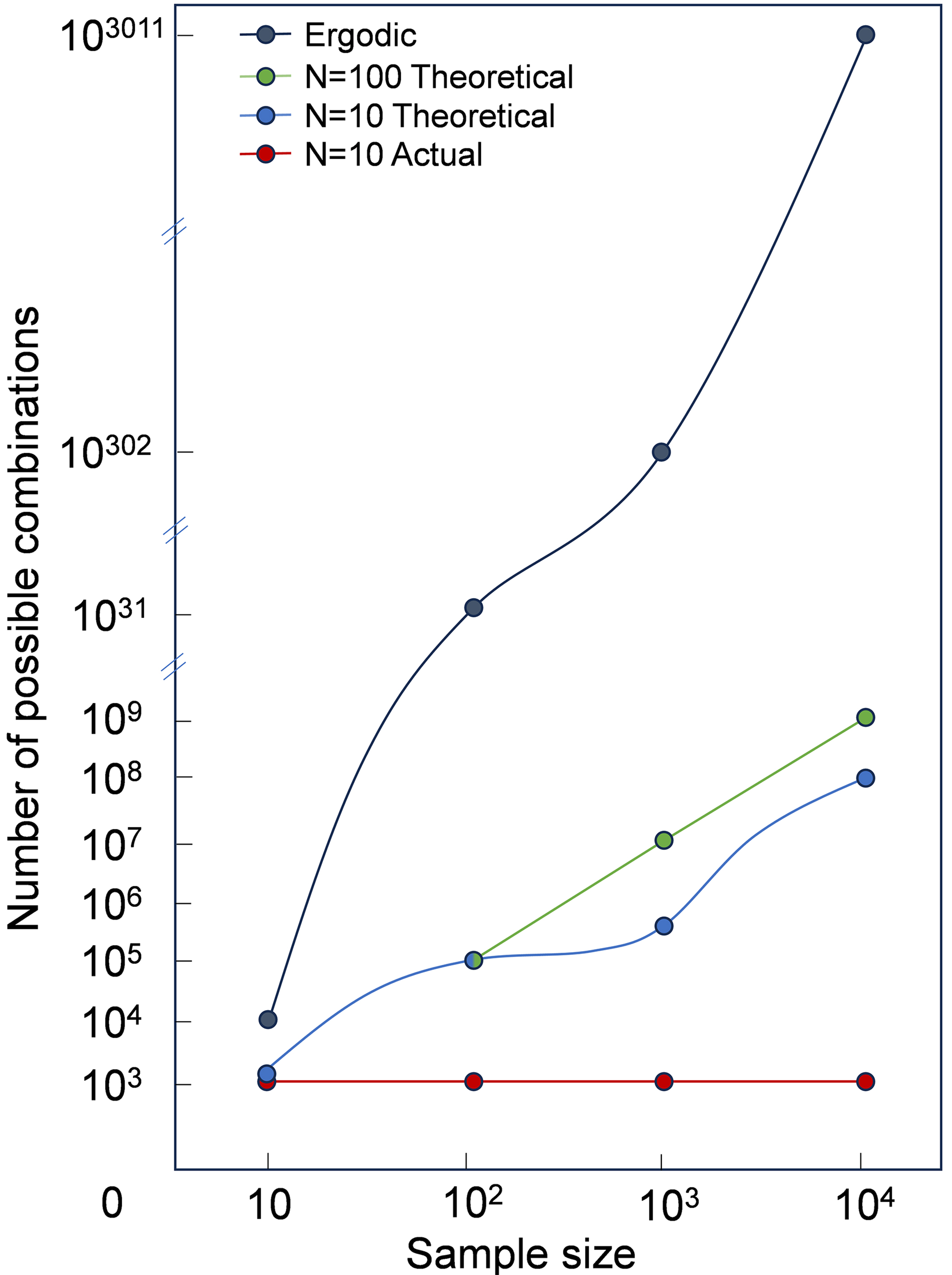
Figure 8. DSMR framework retrieval efficiency analysis diagram. DSMR: Data screening and model retrieval framework based on active learning.
While traversal allows for a wider range of data selection and combination methods, DSMR has the advantage of utilizing an active learning approach to data calibration, where samples that do not contribute much to the model are not involved in subsequent combinations, and therefore the number of combinations will be smaller. The step size N in DSMR can be adjusted to achieve a balance between accuracy and efficiency. In theory, a larger step size N will result in greater accuracy, but at the cost of reduced computational efficiency. When the quantity of data is considerable, a step size of N equal to 10 computes approximately two to three orders of magnitude fewer combinations than N equal to 100. In practice, when the algorithms and hyperparameter optimization methods are consistent, the data sampling can be bootstrapped by model evaluation. This is demonstrated by the four validation examples, which show that the best model can be found in 10 rounds of iterations. In the practical case where N is 10 and 10 algorithms are available, the total number of computations is only of the order of 103. The efficiency of the DS module data sampling is contingent upon the coupled efficacy of the MR module Bayesian automatic parameter tuning and unmanned intervention. The accuracy and generalization ability of the tuning parameters must be considered, as traversal methods will inevitably result in a certain degree of precision loss. To circumvent this, the data will be randomly disrupted in each iteration for multiple calculations. These results will then be combined with cross-validation to identify the optimal outcome, thereby ensuring that the data is fully explored. In conclusion, the DSMR framework employs an active learning-based reduction/increase data sampling strategy, which effectively identifies the most effective samples for the model by reducing redundant samples, selecting data points with high information gain, and optimizing the data distribution to maximize the learning effect, accelerating the learning process of the model and improving the generalization performance, particularly in the case of scarce data or expensive annotations. The iterative process of active learning enables the updating of decision boundaries and the calibration of confidence in samples. This then permits the selection of the most valuable samples from the unlabeled dataset for the next round of training.
Besides, the framework can be used in a low-code, automated way. Users only need to input data in CSV format, select algorithms, evaluation metrics, and data optimization steps, and then output performance metrics and model ontology. The framework uses statistical machine learning algorithms and Bayesian optimization based on scikit-learn, a machine learning library that comes with Python. DSMR performs computations using the CPU (Intel i7-14700KF), and its computational efficiency depends on the data volume, the range of hyperparameters, and the number of data splits. The larger or broader these factors are, the more computation time is required. For example, using the Wen-HV dataset with 273 entries, a relatively small hyperparameter range, and splitting the data into only 10 subsets, a single iteration takes approximately 8 h. Typically, the relatively optimal model (compared to the baseline models in the literature) can be found within 10 iterations. The statistical machine learning approach is suitable for material datasets with limited data volume, and we will continue to improve it by introducing deep learning to make the framework suitable for different levels of data. In conclusion, we are dedicated to the continuous improvement and distribution of DSMR, with the objective of resolving the issues associated with model construction in materials design. This encompasses the selection of high-quality data subsets, the automation of model construction through low-code techniques, and the optimization of materials data management. We posit that DSMR has the potential to become a vital tool for materials design, particularly for researchers lacking in programming expertise, and to drive advances in materials informatics.
CONCLUSIONS
In conclusion, the DSMR framework addresses the critical challenge of efficiently navigating the vast search space of data subsets, algorithms, and hyperparameters in materials science. Through active learning, it successfully identifies better models while restructuring complex external data. The framework demonstrated exceptional performance across diverse materials datasets, achieving 3.3%-10.3% improvement over state-of-the-art results in the literature, including a remarkable 10.3% error reduction for AlCoCrCuFeNi hardness prediction and 42.6% improvement through external data integration. DSMR strikes an ideal balance between computational efficiency and predictive accuracy, while its low-code implementation enhances accessibility for materials researchers. This framework represents a significant advancement in materials informatics, providing a powerful tool for accelerating materials design and discovery through intelligent data management and model optimization.
DECLARATIONS
Authors’ contributions
Conceived and designed the experiments, performed the experiments, analyzed the data, contributed materials/analysis tools, wrote the paper: Chen, J. (Jianhua Chen)
Analyzed the data, contributed materials/analysis tools: Chen, J. (Junwei Chen); Zhao, B.
Provided guidance on the editing and funding support: Fan, Y.
Conceived and designed the experiments, analyzed the data, contributed materials/analysis tools, wrote the paper: Yu, Z.
Conceived and designed the experiments, analyzed the data, contributed materials/analysis tools: Luan, J.
Conceived and designed the experiments, provided guidance on the editing and funding support: Chou, K.
Availability of data and materials
More raw details and tutorials are also available from Supplementary Materials. The program and source codes of the DSMR framework are available (https://github.com/Mat-Design-Yu/DSMR).
Financial support and sponsorship
The authors are especially grateful to the financial support by the Aeronautical Science Foundation of China (No. 2023Z0530S6005), the National Natural Science Foundation of China (No. 52274301), the National Key Research and Development Program of China (No. 2023YFB3712401), Academician Workstation of Kunming University of Science and Technology (2024), Ningbo Yongjiang Talent-Introduction Programme (No. 2022A-023-C) and Zhejiang Phenomenological Materials Technology Co., Ltd., China.
Conflicts of interest
All authors declared that there are no conflicts of interest.
Ethical approval and consent to participate
Not applicable.
Consent for publication
Not applicable.
Copyright
© The Author(s) 2025.
Supplementary Materials
REFERENCES
1. Rao, Z.; Tung, P. Y.; Xie, R.; et al. Machine learning-enabled high-entropy alloy discovery. Science 2022, 378, 78-85.
2. Chen, J.; Zhang, Y.; Luan, J.; et al. Prediction of thermal conductivity in multi-component magnesium alloys based on machine learning and multiscale computation. J. Mater. Inf. 2025, 5, 22.
3. Yuan, Y.; Sui, Y.; Li, P.; Quan, M.; Zhou, H.; Jiang, A. Multi-model integration accelerates Al-Zn-Mg-Cu alloy screening. J. Mater. Inf. 2024, 4, 23.
4. Chen, C.; Zuo, Y.; Ye, W.; Li, X.; Deng, Z.; Ong, S. P. A critical review of machine learning of energy materials. Adv. Energy. Mater. 2020, 10, 1903242.
5. Hu, M.; Tan, Q.; Knibbe, R.; et al. Recent applications of machine learning in alloy design: a review. Mater. Sci. Eng. R. Rep. 2023, 155, 100746.
6. Wen, C.; Zhang, Y.; Wang, C.; et al. Machine learning assisted design of high entropy alloys with desired property. Acta. Mater. 2019, 170, 109-17.
7. Li, S.; Li, S.; Liu, D.; Zou, R.; Yang, Z. Hardness prediction of high entropy alloys with machine learning and material descriptors selection by improved genetic algorithm. Comput. Mater. Sci. 2022, 205, 111185.
8. Zhang, Y.; Ren, W.; Wang, W.; et al. Interpretable hardness prediction of high-entropy alloys through ensemble learning. J. Alloys. Compd. 2023, 945, 169329.
9. Altmann, A.; Toloşi, L.; Sander, O.; Lengauer, T. Permutation importance: a corrected feature importance measure. Bioinformatics 2010, 26, 1340-7.
10. Darst, B. F.; Malecki, K. C.; Engelman, C. D. Using recursive feature elimination in random forest to account for correlated variables in high dimensional data. BMC. Genet. 2018, 19, 65.
12. Shlens, J. A tutorial on principal component analysis. arXiv 2014, arXiv:1404.1100. https://doi.org/10.48550/arXiv.1404.1100. (accessed 19 Jun 2025).
13. Zhang, H.; Fu, H.; He, X.; et al. Dramatically enhanced combination of ultimate tensile strength and electric conductivity of alloys via machine learning screening. Acta. Mater. 2020, 200, 803-10.
14. Jiang, L.; Fu, H.; Zhang, H.; Xie, J. Physical mechanism interpretation of polycrystalline metals’ yield strength via a data-driven method: a novel Hall–Petch relationship. Acta. Mater. 2022, 231, 117868.
15. Gupta, S.; Gupta, A. Dealing with noise problem in machine learning data-sets: a systematic review. Procedia. Comput. Sci. 2019, 161, 466-74.
16. Mohammed, R.; Rawashdeh, J.; Abdullah, M. Machine learning with oversampling and undersampling techniques: overview study and experimental results. In 2020 11th International Conference on Information and Communication Systems (ICICS), Irbid, Jordan. Apr 07-09, 2020. IEEE; 2020. pp. 243-8.
17. Li, K.; Persaud, D.; Choudhary, K.; DeCost, B.; Greenwood, M.; Hattrick-Simpers, J. Exploiting redundancy in large materials datasets for efficient machine learning with less data. Nat. Commun. 2023, 14, 7283.
18. Chen, S.; Cao, H.; Ouyang, Q.; Wu, X.; Qian, Q. ALDS: an active learning method for multi-source materials data screening and materials design. Mater. Design. 2022, 223, 111092.
19. Frazier, P. I. Bayesian optimization. In: Gel E, Ntaimo L, Shier D, Greenberg HJ, editors. Recent advances in optimization and modeling of contemporary problems. INFORMS; 2018. pp. 255-78.
20. Shahriari, B.; Swersky, K.; Wang, Z.; Adams, R. P.; de Freitas, N. Taking the human out of the loop: a review of Bayesian optimization. Proc. IEEE. 2016, 104, 148-75.
21. Pedregosa, F.; Varoquaux, G.; Gramfort, A.; et al. Scikit-learn: machine learning in Python. J. Mach. Learn Res. 2011, 12, 2825-30. https://www.jmlr.org/papers/volume12/pedregosa11a/pedregosa11a.pdf?source=post_page. (accessed 19 Jun 2025).
22. Chen, T.; Guestrin, C. XGBoost: a scalable tree boosting system. arXiv 2016, arXiv:1603.02754. https://doi.org/10.48550/arXiv.1603.02754. (accessed 19 Jun 2025).
23. Prokhorenkova, L.; Gusev, G.; Vorobev, A.; Dorogush, A. V.; Gulin, A. CatBoost: unbiased boosting with categorical features. arXiv 2017, arXiv:1706.09506. https://doi.org/10.48550/arXiv.1706.09516. (accessed 19 Jun 2025).
24. Jo, J. M. Effectiveness of normalization pre-processing of big data to the machine learning performance. J. Korea. Inst. Electron. Commun. Sci. 2019, 14, 547-52.
25. Wong, T. Performance evaluation of classification algorithms by k-fold and leave-one-out cross validation. Pattern. Recognit. 2015, 48, 2839-46.
26. Fushiki, T. Estimation of prediction error by using K-fold cross-validation. Stat. Comput. 2011, 21, 137-46.
27. Ye, Y.; Li, Y.; Ouyang, R.; Zhang, Z.; Tang, Y.; Bai, S. Improving machine learning based phase and hardness prediction of high-entropy alloys by using Gaussian noise augmented data. Comput. Mater. Sci. 2023, 223, 112140.
28. Ma, J.; Cao, B.; Dong, S.; et al. MLMD: a programming-free AI platform to predict and design materials. npj. Comput. Mater. 2024, 10, 1243.
29. Kano, S.; Yang, H.; Suzue, R.; et al. Precipitation of carbides in F82H steels and its impact on mechanical strength. Nucl. Mater. Energy. 2016, 9, 331-7.
30. Williams, C. A.; Hyde, J. M.; Smith, G. D.; Marquis, E. A. Effects of heavy-ion irradiation on solute segregation to dislocations in oxide-dispersion-strengthened Eurofer 97 steel. J. Nucl. Mater. 2011, 412, 100-5.
31. Haertling, G. H. Ferroelectric ceramics: history and technology. J. Am. Ceram. Soc. 1999, 82, 797-818.
32. Green, M. A.; Ho-Baillie, A.; Snaith, H. J. The emergence of perovskite solar cells. Nature. Photon. 2014, 8, 506-14.
33. Correa-Baena, J. P.; Saliba, M.; Buonassisi, T.; et al. Promises and challenges of perovskite solar cells. Science 2017, 358, 739-44.
34. Chen, X.; Wang, Q.; Cheng, Z.; et al. Direct observation of chemical short-range order in a medium-entropy alloy. Nature 2021, 592, 712-6.
35. Zhang, R.; Zhao, S.; Ding, J.; et al. Short-range order and its impact on the CrCoNi medium-entropy alloy. Nature 2020, 581, 283-7.
36. Shi, P.; Li, R.; Li, Y.; et al. Hierarchical crack buffering triples ductility in eutectic herringbone high-entropy alloys. Science 2021, 373, 912-8.
37. Senkov, O.; Senkova, S.; Woodward, C. Effect of aluminum on the microstructure and properties of two refractory high-entropy alloys. Acta. Mater. 2014, 68, 214-28.
38. Guo, S. Phase selection rules for cast high entropy alloys: an overview. Mater. Sci. Technol. 2015, 31, 1223-30.
39. Zhang, Y.; Wen, C.; Wang, C.; et al. Phase prediction in high entropy alloys with a rational selection of materials descriptors and machine learning models. Acta. Mater. 2020, 185, 528-39.
Cite This Article
How to Cite
Download Citation
Export Citation File:
Type of Import
Tips on Downloading Citation
Citation Manager File Format
Type of Import
Direct Import: When the Direct Import option is selected (the default state), a dialogue box will give you the option to Save or Open the downloaded citation data. Choosing Open will either launch your citation manager or give you a choice of applications with which to use the metadata. The Save option saves the file locally for later use.
Indirect Import: When the Indirect Import option is selected, the metadata is displayed and may be copied and pasted as needed.
About This Article
Special Issue
Copyright

Data & Comments
Data
0


Comments
Comments must be written in English. Spam, offensive content, impersonation, and private information will not be permitted. If any comment is reported and identified as inappropriate content by OAE staff, the comment will be removed without notice. If you have any queries or need any help, please contact us at support@oaepublish.com.