Uncertainty aware design space modeling for sample efficiency in material design of bainitic steels

Design problem

In the present work, we are modeling the design space of CFB steels. In this steel type, the carbide precipitation is suppressed during bainitic transformation by adding silicon ^[24] or aluminum ^[25,26], and it is defined as having at least 1 wt.% silicon. The retained austenite is stabilized by carbon, which is redistributed during the bainitic transformation from bainitic ferrite to retained austenite ^[14]. We place a lower limit of carbon concentration to ensure some retained austenite. Additionally, considered alloying elements are Si, Mn, Cr, Mo, Al and V, excluding critical raw elements such as Ni, W and Co [Table 1]. Furthermore, CFB steel is intended to exhibit relatively low overall alloying content. Therefore, the total concentration of alloying elements, denoted as $$ \sum_{\text{wt.%}} $$, is restricted to a maximum of 10 wt.%. We decided to focus on two representative processes: isothermal holding or austempering which is shown in Figure 1A and continuous cooling which is shown in Figure 1B.

Figure 1. Temperature profile (in black) for the processes leading to the formation of CFB, along with time/temperature regions where constraints apply: (A) isothermal holding (austempering) and (B) continuous cooling. Colored regions indicate phases: Ferrite/Pearlite (F/P), Bainite (B), and Martensite (M). The constraints are enumerated by C1-C7. CFB: Carbide-free bainite.

As illustrated schematically, the sample is heated up to an austenitization temperature, typically above 800 ℃ and held for a duration $$ t_\text{A} $$ to obtain the high-temperature phase of steel, austenite (A). Subsequently, the sample is either rapidly and continuously cooled to an isothermal holding temperature $$ T_{\text{iso}} $$ or continuously cooled directly to room temperature with a cooling rate $$ \dot{T} $$ to obtain ferrite/Pearlite (F/P), bainite (B), martensite (M) microstructures or a mixture of both. Both processes have an upper time limit: the isothermal process is limited by a maximum holding time $$ \max(t_{\text{iso}}) $$, while the continuous cooling process is limited by a maximum cooling rate $$ \max(\dot{T}) $$. This defines the search space in the present work, which is summarized in Table 1.

The requirement for the sample to be only bainitic (B) can be expressed by a list of constraints, which are listed below and, if applied to the search space, yield the design space. As can be seen in Figure 1, both processes have windows for the process parameters, which are composition-dependent.

Data generation for C1 - homogeneity of austenitization

The stability and occurrence of carbides, austenite, and ferrite phase is modeled in thermodynamic databases. The MatCalc Software^[28] and database (mc_fe version 2.061 ^[39]) are used to calculate equilibrium temperature scans for a surrogate model to increase in evaluation speed. The MatCalc simulation considers the following phases in the scan for the austenitization temperature: liquid, austenite, ferrite, cementite, and several other carbides (M6C, M7C3, M23C6, LAVES_Phase, K_CARB, and FCC_A1#01). For each alloy composition, a temperature scan of equilibrium calculations is performed starting at a temperature of 1,873 ℃ and a step size of 2 ℃.

Evaluation of carbon redistribution for C4

For a given isothermal holding temperature ($$ T $$), the retained austenite during bainitic transformation is enriched with carbon until a maximum $$ w_C(T) $$, at which point the driving force for the transformation is completely consumed. This can be interpreted as the bainite start temperature of the alloy with the enriched carbon concentration

The carbon enrichment of the retained austenite stabilizes it against martensite transformation during cooling to room temperature. This explains the difference between the martensite start of the initial alloy $$ M_{S}(w_{C, 0}, \{w\}) $$ and of the retained austenite $$ M_{S, RA}(w_{C}(T), \{x\}) $$. Both are modeled similarly, but for the retained austenite, the carbon enrichment $$ w_C(T) $$ must be predicted. This can be done with a bainite start model (C2), but the model is strongly extrapolated for carbon concentrations. Therefore, the best-performing physical-based displacive bainite start model from Ref. ^[31] paired with the mc_fe version 2.061 database ^[39] is used for the prediction.

Experimental data

The data used in this work consists of experimental data from literature, as well as experimental data produced in this work. The experimental details for the production of the samples are described in Ref. ^[31]. The alloys were fabricated using a high-frequency remelting furnace (HRF), the "PlatiCast-600-Vac," from the Linn High Therm GmbH, Germany ^[40,41]. Approximately 450 g of each alloy, shaped into 26.5 mm × 26.5 mm × 90 mm ingots, was melted using high-purity raw materials. The process took place in a pure alumina crucible under an argon atmosphere at five atmospheres overpressure. The molten material was centrifugally cast into a cold copper mold, resulting in highly homogeneous samples due to the combination of inductive melting, centrifugal casting, and rapid solidification.

Chemical composition analyses, detailed in Table 2, are performed using optical emission spectroscopy (OES, model OBLF QSG 750). To ensure a consistent initial microstructure, the raw samples underwent heat treatment in an argon-purged chamber furnace. This included diffusion annealing at 1,200 ℃ for four hours, achieved with a heating rate of 300 ℃/s. Following this, the samples were removed from the furnace and allowed to cool freely to room temperature. To further refine the coarse-grained microstructure, a normalization annealing was conducted at 960 ℃ - at least 50 ℃ above the previously calculated Ae3 temperature - for 50 min, followed by free cooling to room temperature. Metallographic examination of the resulting ingots confirmed a uniform microstructure.

Cylindrical dilatometer samples with a diameter of 4 mm and a length of 10 mm are produced. The heat treatment and measurement is done with a TA Instruments DIL 805 A dilatometer in vacuum. The samples are austenitized for 30 min at 960 ℃ with a heating rate of 2 K/s. The bainite start temperature was measured for selected compositions, with the methods described in Ref. ^[31]. The region of carbide free bainitic steels was determined with various isothermal and continuous cooled experiments by observing the region of ferrite/pearlite and martensite.

The evaluation of the martensite start temperature of the initial alloy, the martensite start temperature of the retained austenite phase and the occurrence of the F/P phase is done with the tangent method ^[42] and supported by metallography.

ML models

The ML models used in this work include Gaussian process regression (GPR) ^[43,44], linear regression, polynomial regression, logistic regression, RFs ^[45], gradient boosting machines [XGBoost, light gradient boosting machine (LGBM)] ^[46,47], NNs ^[48], monotone NNs^[49], and SVM^[50]. A full list can be seen in Table 3. There are fundamentally two types of models: local models, which predict the target based on its proximity to neighboring data points, and global models, which capture overarching trends in the data.

Each of the constraints (C1 to C6) corresponds to a classification problem, where the task is to determine whether the input sample should be accepted or rejected. However, the way experimental data is reported in the literature, combined with the nature of the experiments producing this data, results in a significant class imbalance. For example, more data points are reported with a transformation time of less than three hours than with a time greater than three hours, due to the high cost of the experiments. Thus, we use regression models to predict continuous values for constraints C2 to C6, which are then thresholded to classify the samples into binary categories (accept/reject).

Except for C1, where data is sampled from a thermodynamic model, no physics-based models for the remaining constraints significantly outperform ML approaches. Since this work evaluates points across the entire search space defined in Table 2, the model operates in an extrapolative regime, which presents challenges in ensuring reliable predictions beyond the training domain. For constraints C2 to C5, we assume that the quantities follow (at least approximately) a general trend and exhibit monotonicity. For example, if an alloy with 2 wt.% Mn fails to satisfy constraint C4, increasing Mn to 4 wt.% is also assumed to fail C4. This highlights a key challenge for local models, which may struggle to capture such trends in regions with sparse data or when extrapolating beyond the training domain. As a result, global models are better suited for addressing these constraints.

Another issue is the substantial degree of extrapolation required by the models, potentially resulting in inaccurate predictions. Thus, we also require reliable uncertainty estimation to avoid premature exclusion of valid samples. Popular methods for uncertainty estimation include probabilistic and Bayesian approaches (e.g., GPR). One advantage of GPRs with appropriate kernel functions is their ability to express a relationship between distance from the training data and uncertainty ^[51]. In GPR, predictions take the form of a Gaussian distribution $$ \mathcal{N}(\mu(x), \sigma^2(x)) $$, with $$ \mu(x) $$ representing the mean prediction and $$ \sigma^2(x) $$ denoting the variance. We use the standard deviation $$ \sigma(x) $$ as an uncertainty measure, i.e., $$ u(x)=\sigma(x) $$. However, GPR uncertainty estimates are reliable only if the model is well specified ^[20]. This means the chosen kernel, likelihood function, and hyperparameters must align with the true data-generating process. For example, if the kernel fails to match the actual smoothness of the data, the resulting uncertainty estimates become unreliable. Unfortunately, this condition is rarely met in practice, requiring additional calibration through CP^[20,22]. In contrast, deterministic algorithms (e.g., RFs, NNs) approximate the training data as $$ \hat{y} = f(x; \theta) $$. They scale efficiently with large datasets and can deliver competitive predictive accuracy. However, they tend to perform poorly in extrapolated regions and lack principled mechanisms for estimating uncertainty. To address this, we assume a uniform uncertainty of $$ u(x)=1 $$ for the full input space, which is then calibrated with CP^[22].

Uncertainty quantification

In this section, we summarize key sources of uncertainty and how CP provides calibrated uncertainty estimates for both probabilistic and deterministic models. Additionally, we augment the uncertainties with distance measures, e.g., Mahalanobis distance, to detect distribution shifts between the training data and data encountered during deployment. This allows us to adjust uncertainty estimates in extrapolated regions. By doing so, the uncertainty estimates are based on the proximity of the current input to the training data. This adaptation is especially useful for deterministic models, where we initially assume constant uncertainty.

Prediction uncertainties can arise from several sources ^[52,53], each representing a distinct type of uncertainty, as illustrated in Figure 2. Figure 2A stems from the inherent variability or noise in the data. This uncertainty is caused by random variations or measurement uncertainties, as shown by the scattered data points around the true function.

In contrast, Figure 2B originates from the model’s limited understanding of the data-generating process, e.g., when the model is underfitting the data and is unable to capture the complexity of the underlying function. Additionally, Figure 2C occurs when there is a mismatch between training and test distributions, e.g., when certain regions of the input space are sparsely sampled or fall outside the range of the training data (i.e., extrapolation regions). In such cases, the model exhibits higher uncertainty in underrepresented areas, reflecting its limited knowledge. Accounting for this uncertainty is crucial to prevent overconfident predictions in unexplored regions of the design space, which are underrepresented in the training data. Failure to address this issue may lead to the premature exclusion of potentially valuable compositions. In the following, we describe our proposed method to account for such sources of uncertainty.

Figure 2. Illustrations of different types of uncertainty in model predictions.

To quantify prediction uncertainty, we employ prediction intervals, which define the range within which the true value is expected to fall with a specified probability, $$ \alpha $$. Consider the training data $$ (x_i, y_i) \in \mathcal{D} $$ for $$ i = 1, \dots, n $$, where $$ x_i $$ represents the input features and $$ y_i $$ the target values. Given a confidence level $$ \alpha $$, the prediction interval $$ \mathcal{C}_\alpha $$ for a new input $$ x^* $$ is defined by

Uncertainty quantification methods often fail to guarantee such calibrated prediction intervals, i.e., intervals that reliably contain the true value with the stated probability ^[54]. Even GPR, an established probabilistic method for uncertainty estimation, produces uncalibrated prediction intervals in practice due to model misspecification^[20,55].

CP

CP^[21,22,56] calibrates prediction intervals from an uncertainty heuristic $$ u(x) $$ (e.g., predictive variance from a GPR), making no assumptions about the underlying data distribution. CP provides prediction intervals with a user-specified coverage probability ($$ \text{cov} $$) (e.g., 90%), given that the data satisfies the assumption of exchangeability. Exchangeable data means that the order of the data points does not affect their joint distribution. In simpler terms, exchangeability assumes that the data points are drawn from the same process and treated symmetrically, without requiring the stricter independent and identically distributed (i.i.d.) assumption.

To illustrate the CP workflow, Figure 3 compares two uncalibrated uncertainty heuristics, the calibration process through CP, and the resulting calibrated uncertainty estimates. Figure 3A shows overconfident estimates $$ u_1(x) $$, where intervals are too narrow and fail to capture the variability of the data, underestimating the uncertainty. On the other hand, the uncertainty estimates $$ u_2(x) $$ in Figure 3B are underconfident. The intervals are excessively wide, leading to overestimation of uncertainty. Both cases highlight the need for calibration to achieve intervals that accurately reflect the desired coverage. The key idea of CP calibration is to scale the uncertainty heuristic scores of the unseen test data by a calibration factor $$ \hat{q} $$ to obtain the prediction intervals. The calibration factor $$ \hat{q} $$ in our example is chosen such that the prediction intervals have a $$ \text{cov} $$ of $$ \alpha = 90% $$. Due to its efficiency and simplicity, the most commonly used CP method in practice is split CP^[57]. This approach divides the data into a proper training set and a calibration set. In the following, we outline the steps for implementing split CP^[22].

Figure 3. Calibration of uncertainty estimates using CP. Overconfident (A) and underconfident (B) prediction intervals are scaled with the split CP framework (C and D) to achieve a specified coverage with tight bounds (E and F). CP: Conformal prediction.

1. We select an uncertainty heuristic $$ u(x) $$ [e.g., GPR standard deviation $$ \sigma(x) $$, or uniform $$ u(x)=1 $$].

2. Next, we calculate the deviation between the model’s predictions and the true observed values on a separate calibration set. For regression tasks, we compute residuals $$ r(x_i, y_i) = |y_i - f(x_i)| $$, with $$ f(x_i) $$ representing the model’s prediction for input $$ x_i $$. This results in the non-conformity scores $$ s(x_i, y_i) = \frac{r(x_i, y_i)}{u(x_i)} $$. For classification tasks, we use the predicted probabilities for each class $$ c $$, denoted as $$ \hat{p}_c(x_i) $$. The non-conformity score is the predicted probability for the correct label $$ y $$, $$ s(x_i, y_i) = \hat{p}_{y_i}(x_i) $$.

3. We compute the calibration factor $$ \hat{q}_\alpha $$ as the $$ \frac{\lceil{(m+1)\alpha}\rceil}{m} $$ quantile of the scores $$ s(x_i, y_i) $$, where $$ m $$ is the number of samples in the calibration dataset.

4. For regression models, the prediction intervals are constructed as $$ \mathcal{C}_\alpha(x^*) = [f(x^*) - u(x^*) \hat{q}_\alpha, \; f(x^*) + u(x^*)\hat{q}_\alpha] = [q_{l}, q_{u}] $$. For classification models, the prediction set is obtained as $$ \mathcal{C}_\alpha(x^*) = \{y: \hat{p}_y(x^*) \geq \hat{q}_\alpha \} $$.

For $$ u_1(x) $$, calibration adjusts the overly narrow intervals, scaling them to meet the desired 90% coverage. For $$ u_2(x) $$, calibration scales down the excessively wide intervals, achieving the same width as those for $$ u_1(x) $$, while maintaining valid coverage.

Modeling workflow and metrics

The modeling workflow, illustrated in Figure 4, evaluates prediction models and distance estimators for computing the constraints (C1-C4, C6). Due to the limited size of the experimental datasets [Table 4], we adopt a 10-fold cross-validation strategy to select the optimal prediction and distance model. The dataset is split into training and test sets, with the test set used exclusively for computing performance metrics. The split is performed based on materials (same alloy compositions), ensuring that no material in the test set overlaps with the training set. For regression tasks with limited data (C2-C6), we improve cross-validation robustness by stratifying based on discretized target with five bins, ensuring a balanced representation across folds to improve model robustness and generalization. Thus, we avoid overly optimistic results by evaluating the model’s ability to extrapolate to novel material compositions, rather than predicting changes driven solely by treatment temperature variations. Table 4 summarizes the number of materials, and the number of total data samples for each constraint. Each training fold is further divided into a "proper training set" and a "calibration set" used for CCP (5-folds). The prediction model is trained using the proper training set only, avoiding contamination of the calibration set used for CP.

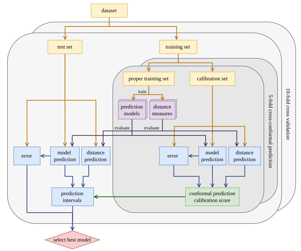
Figure 4. Overview of the model selection and evaluation process for the ML models and distance-aware cross-CP. ML: Machine learning; CP: conformal prediction.

To address prediction target variation across several orders of magnitude - such as bainite transformation times (C4) and critical cooling rates (C6) - we apply a base-10 logarithmic transformation

where $$ y_{i, \text{data}} $$ are the original and $$ y_{i} $$ are transformed values. This transformation reduces the scale of the targets, ensuring that error metrics emphasize relative differences over absolute magnitudes.

Experimental results

The combined experimental results for the sample produced in the present work are listed in Table 2 and shown in Figure 5. The experimental uncertainty for the martensite start temperature of the initial alloy is 20 ℃; for the retained austenite it is 30 ℃, and for the logarithmic transformation times it is 0.2 log(s). The martensite start temperature (M_S) of the initial alloy is indicated by a dashed blue line on both temperature axes, serving as a reference. This temperature defines the lower limit of the isothermal holding temperatureT_iso, with the restricted region of T_iso shaded in red. On the vertical axis, the martensite start temperature of the retained austenite M_{S, RA} is shown in blue. The bainite start temperatures of the alloys, already published in Ref. ^[31], are indicated as green dashed lines. At the bainite start temperature B_S, no bainite forms, resulting in M_S= M_{S, RA}. As the temperature decreases, carbon enrichment occurs, leading to a stabilizing effect that lowers the martensite start temperature. This decrease continues until the martensite start temperature falls below the detection limit. For consistency, these undetectable points are marked at 50 ℃ in Figure 5. This trend is observed across all produced samples.

Figure 5. Experimental results for logarithmic bainitic transformation time $$ \log_{10}(t_{\text{90%}}) $$, the martensite start temperature of the initial alloy $$ M_{\text{S}} $$ and the martensite start temperature of the retained austenite $$ M_{\text{S, RA}} $$. For $$ M_{\text{S, RA}} $$ under the detection limit of 50 ℃, it is drawn at 50 ℃. The combination of these measurements gives the process window for CFB steel, visualized with the green area. CFB: Carbide-free bainitic.

The bainitic transformation time spans several orders of magnitude due to the strong influence of material composition and thermodynamic parameters on the kinetics of the phase transformation. To better illustrate this behavior, log₁₀(t_90%) represents the time required to achieve 90% of the bainitic transformation, which is illustrated in Figure 5. This logarithmic representation provides a clearer comparison of the transformation times across different samples.

The transformation times typically exhibit a characteristic C-shaped behavior, which can be observed in several of the samples. Samples S1 to S5, for example, were specifically designed to study the effect of varying carbon content on transformation kinetics. As shown in Figure 5, increasing the carbon content leads to a significant increase in transformation time. For samples S14, S17, and S18, the bainitic phase transformation did not complete at any isothermal holding temperature, leaving the martensite start temperature (M_S) of the initial alloy as the only usable data point. The composition of S14 is identical to that of S7, except for an increased manganese content. This difference highlights the strong influence of manganese on transformation kinetics, as its presence significantly delays the bainitic transformation. The too slow transformation kinetics of S17 and S18 can be explained by their very high carbon content of over 1 wt.%. For the remaining samples, no clear correlation between transformation time and material composition is evident.

The process window for CFB steels, highlighted in green in Figure 5, is defined by the following conditions: The isothermal holding temperature exceeding the martensite start temperature, the martensite start temperature of the retained austenite being below the detection limit, and the transformation completing within 10,800 s. The region between the red and green areas represents a high probability that the isothermal holding temperature within this range will also produce carbide-free bainite. However, this assumption has not been experimentally validated. Depending on the material composition, the process window can vary significantly: it can be quite large (e.g., for samples S9, S11, and S13) or even non-existent (e.g., for samples S14, S17 and S18).

Dataset

The primary classification task in this study is to determine whether the steel type is CFB for a given chemical composition and heat treatment parameters. However, by decomposing the problem into multiple constraints, the available data for each constraint can be expanded by incorporating data from other steel groups, assuming that the underlying physical phenomena are consistent. For instance, the formation of ferrite or pearlite is not influenced by whether or not bainite is subsequently formed. Similarly, the bainite start temperature is independent of whether the steel is bainitic or CFB.

The dataset and models utilized in this study are publicly accessible through the associated Zenodo repository (Code and datasets will be published upon acceptance). The dataset for the austenitization condition is produced with MatCalc on a grid with eight grid points for each dimension and the limits listed in Table 2. The total alloy content limit $$ \sum_{\text{wt.%}} $$ of 10 wt.% is enforced beforehand, which reduces the number of grid points from $$ 8^7 $$ one-third to about 800,000.

For the bainite start temperature, the dataset is taken from Ref. ^[31]. The dataset for martensite start temperatures $$ M_{\text{S}} $$ is derived from a comprehensive collection in Ref. ^[33] combined with experimental data from the present work. For the martensite start temperature of the retained austenite, the dataset from the normal martensite start temperature is used, combined with experimental data from the present work with adapted carbon concentration according to the description in the methods. Bainitic transformation times are obtained by digitizing bainitic phase transformation curves from the Refs. ^[63–80] and experimental data from the present work. The literature data for ferrite transformation times was digitized from steel transformation time atlases^[81–83]. For all datasets, feature selection was performed to refine the dataset, excluding features or elements with insufficient entries or concentrations too low to have a measurable influence on the targets.

The constraints are a combination of material-specific quantities, which depend solely on composition (C1, C2, C3, C6), and process-dependent quantities (C4, C5). For the process-dependent quantities, this leads to a dataset that is sparse across most dimensions, except for temperature. To provide a clearer representation of the datasets, the number of materials, the number of data points and additional features to C, Si, Mn, Cr, Mo, Al, V and $$ T_{\text{iso}} $$ for all constraints are summarized in Table 4.

Modeling results

With the datasets presented in Table 4, we assess the performance of the different ML models listed in Table 3 with 10-fold cross-validation. For each constraint, the best-performing model is selected for subsequent investigations.

The first condition C1, austenitization, is a classification task. The training data is obtained from simulations, and the ML models act as surrogate models to replace time-intensive simulations for novel input compositions. The results for the different ML models are summarized in Table 5, with NNs achieving over 97% accuracy on the test set splits, and the desired $$ \text{cov} $$ of 90%. Figure 6A illustrates the calibration curve and confusion matrix for NNs. The predicted probabilities closely align with the true probabilities, as indicated by the calibration curve (blue solid line) and the perfectly calibrated line (black dashed line). Additionally, the confusion matrix shows the performance of the classifier, with 63.82% of samples correctly classified as invalid, 32.28% correctly classified as valid, and minor misclassifications in the remaining categories.

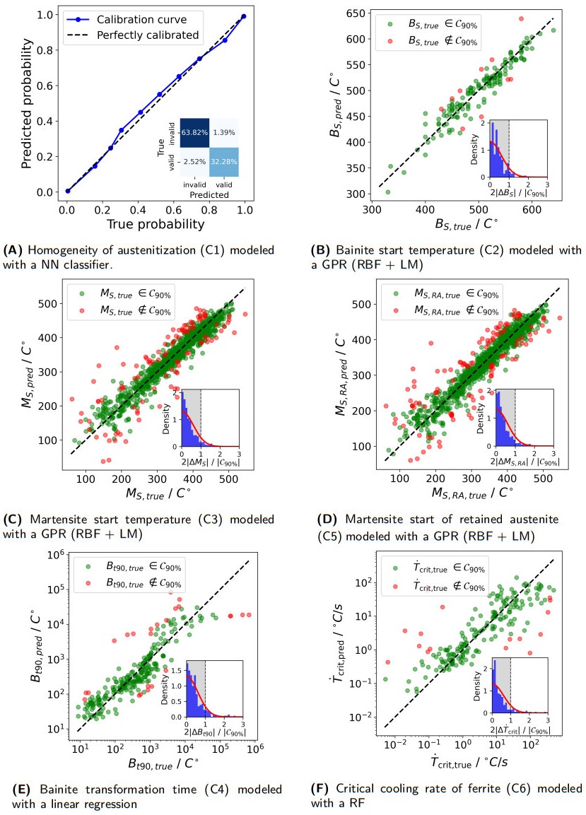
Figure 6. Calibration curve and confusion matrix for the classification task (C1). Predicted test values versus true values for the constraints treated as regression problems (C2-C6).

For the other constraints, the training data is sourced from experimental results, introducing a higher degree of variability and uncertainty compared to purely simulation-based data as is the case for C1. Additionally, the data does not span the entire design space, requiring the models to extrapolate. To account for distribution shifts, we use distance-aware CP.

The bainite start temperature (C2), martensite start temperature (C3), and martensite start temperature of the retained austenite (C5) are grouped together as they all focus on a transition temperature. For these constraints, we assume that the problem is monotonic with respect to each alloy element. The performance of the ML regression models is listed in Tables 6-8. The test prediction performance of the best ML regression models is shown in Figure 6B-D. Green points correspond to predictions within the 90% coverage region ($$ C_{90\%} $$), while red points indicate predictions outside this region. The dashed black line represents perfect agreement between predicted and true values. The histogram shows the distribution of prediction errors scaled by uncertainty. These models showing the best performance are used for the final evaluation on the whole design space.

When comparing the results for C2, C3 and C5, it is important to consider that we report results for local and global models shown in Table 3. However, local methods are less desirable due to their poor extrapolation behavior beyond the training data. Tree-based models (RF and LGBM) extrapolate using piecewise constant behavior in regions without training data. Also, GPR with an RBF kernel reverts back to the mean of the training data when extrapolating. Both behaviors fail to account for the physical constraints inherent in the system. For GPR with an RBF kernel, this limitation can be addressed by implementing a linear mean (LM) function, ensuring better alignment with the physical knowledge of the constraints. For the three constraints, the inclusion of quadratic features in polynomial regression has led to worse performance compared with linear regression, which can be attributed to overfitting. The coverage for all constraints and models remains close to the desired 90%, validating the reliability of CP. GPR with an RBF kernel and LM shows the best performance in terms of the MAE and the smallest PIW, for all three constraints. It combines the flexibility of local models (such as GPR with RBF, RF, and LGBM), which on average outperform global models, with the ability of global models to effectively capture broader trends. We selected the GPR with an RBF kernel and LM because of the lower MAE and PIW for the final evaluation for these cases. The similarity in model results for the two martensite start temperature problems is expected because they share a significant fraction of their training data.

A key challenge in modeling the boundary condition C4, i.e., the logarithmic bainite transformation time [log₁₀(t_90%)], is the scarcity of data for transformation times exceeding the 3-hour constraint. This results in limited coverage for long-duration experiments. Additionally, transformation times span several orders of magnitude, necessitating the use of log-transformed targets to stabilize variance and improve model performance. The underlying behavior is monotonic in the chemical elements and has a C-shape in temperature. The results of the ML models are shown in Table 9, and the best-performing model is visualized in Figure 6E. Notably, data points outside the prediction interval are more frequent in regions of high or low transformation times.

While GPR with an RBF kernel achieves the lowest MAE for C4, it struggles with extrapolation, especially when constrained by the limited training data. Assuming that transformation times are approximately monotonic with respect to alloy composition, we can improve linear regression with quadratic temperature features [$$ T^2, \; \log_{10}(T)^2 $$]. Despite achieving a slightly lower $$ R^2 $$, it provides interpretable predictions with stable linear extrapolation and monotonicity, making it the preferred model for deployment in extrapolative regions. Thus, it is selected for the final evaluation. The coverage remained close to the desired 90%. However, the variability of the coverage is higher than in previous tasks, with standard deviations up to 11%, and the width of the prediction interval is relatively large, spanning at least 1.4 orders of magnitude. This can be explained by a suboptimal model performance. As a result, some folds may overestimate or underestimate the uncertainty, especially in regions where data is sparse or the target values span a wide range. Despite this variability, distance-aware CP still demonstrates its robustness by achieving reasonable coverage.

The critical cooling rate of ferrite, i.e., C6, also spans several orders of magnitude. For this reason, similar to the bainite transformation time, predicting $$ \log_{10}(\dot{T}_{\text{crit}}) $$ provides more stability. The predictive performance of the ML regression models is listed in Table 10, and the result of the best model is shown in Figure 6F.

The results for C6 reveal notable variability in the models’ performance. Particularly noteworthy are the performances of the GPR with a polynomial kernel and the NN. Both models exhibit a high MAE, indicating poor predictions for certain data points, despite achieving high coverage and a low PIW. This highlights their failure to accurately predict a few critical samples. Among the evaluated methods, local models such as RFs, XGBoost and GPR achieve the lowest MAE scores of 0.43 ± 0.09, 0.44 ± 0.08, and 0.44 ± 0.1, respectively. This suggests that these models are better suited for capturing the nonlinear relationships in the dataset compared to linear or polynomial regression. The coverage of the CP intervals remains stable across all models, averaging close to the desired 90%, with slight variability due to the relatively small dataset size. Notably, RFs and LGBM perform very similarly; however, because of the higher R² value, the RFs are selected.

To get insight into which features are responsible for the model prediction, SHapley Additive exPlanations (SHAP) analysis is employed ^[84]. The resulting SHAP values quantify the marginal contribution of each feature, where the sign of the SHAP value indicates whether the feature increases or decreases the prediction, and the magnitude reflects the strength of its influence.

The SHAP values for the prediction models are shown in Figure 7. For condition C1 [Figure 7A], high concentrations of aluminum (Al), silicon (Si), and vanadium (V) increase the likelihood of successful austenitization. However, the effect of carbon (C) remains ambiguous. This is attributed to its dual role: while carbon stabilizes austenite and lowers the austenitization temperature into the valid range, it also promotes carbide formation.

Figure 7. SHAP value analysis of models C1 to C6. Subplots (A) to (F) correspond to models C1 to C6, respectively, illustrating the contribution of each feature to the model predictions. SHAP: SHapley Additive exPlanations.

For the bainite start temperature (C2) [Figure 7B], and the martensite start temperatures (C3 and C5) [Figure 7C and D], the SHAP values exhibit a monotonic and approximately linear dependence on concentration, reflecting the LM function of the employed GPR model. Notably, in Figure 7B, carbon does not yield the highest SHAP value despite its substantial influence per wt.%. This discrepancy arises from feature distribution effects within the dataset. A similar pattern is observed for Al and V, which appear less influential due to their limited high-concentration data points.

For bainite transformation time (C4) [Figure 7E], SHAP values highlight manganese (Mn), C, and nickel (Ni) as the dominant factors contributing to prolonged transformation times, while also revealing the nonlinear influence of temperature. Finally, for the critical cooling rate (C6), the SHAP values in Figure 7F indicate complex and inconclusive trends for several elements, particularly for molybdenum (Mo).

Design space

To evaluate the reduction of the design space, the best-performing models for each constraint were applied to $$ 10^6 $$ evaluation points sampled uniformly for the dimensions C, Si, Mn, Cr, Al, V, Mo, $$ T_{\text{iso}} $$ and $$ \log_{10}(\dot{T}_{\text{crit}}) $$ within the boundaries defined in Table 2. In modeling the process-dependent constraints C4 and C5, we implicitly assumed that the isothermal holding temperature complies with constraints C2 and C3. This assumption is grounded in the observation that predicting bainite transformation times above the bainite start temperature is inherently illogical. Furthermore, the formation of martensite before bainite significantly accelerates the bainite transformation process ^[85]. The reduction of the design space was evaluated using three tolerances: low, mid, and high. The mid-tolerance evaluation utilized the mean predictions from the models, while the low tolerance employs the bound of the CP interval which results in a smaller design space, thereby imposing a more stringent constraint. In contrast, the high tolerance evaluation applies the upper bound of the interval, effectively relaxing the constraint. A visualization for the example of C2 ($$ B_{\text{S}} $$) and C3 ($$ M_{\text{S}} $$) is given in Figure 8. For low tolerance, the upper confidence interval for $$ M_{\text{S}} $$ and the lower of $$ B_{\text{S}} $$ is taken, mid-tolerance is evaluated with the mean predictions and high tolerance is evaluated with the lower confidence intervals for $$ M_{\text{S}} $$ and the upper for $$ B_{\text{S}} $$.

Figure 8. Tolerance levels.

The results of these evaluations for both heat treatments are summarized in Figure 9. A significant difference is observed in the percentage of predicted CFB points between the isothermal holding and continuous cooling processes. However, this discrepancy does not reflect the full reality, as the constraint C7, shown in Figure 1, was not incorporated in this study due to missing data. This results in an overestimation of design space. Solving this issue will be part of future work, either by building a data-driven literature model or by direct prediction of bainite transformation kinetics. Furthermore, the increase in space from a higher tolerance level is much larger in the continuously cooled case, which can be explained by the higher uncertainty of constraint C6. At a high tolerance, the C6 constraint does not exclude any test points.

Figure 9. Design space reduction for the different heat treatments; see text for description for tolerance.

For further analysis of the constraints, we focus on the isothermal process and select the high tolerance criterion. This approach uses the calibrated uncertainty intervals to avoid prematurely excluding viable design regions. Even with a high tolerance, the design space is only 20% of the search space, which corresponds to an 80% reduction. The final relationship between each input dimension and the acceptance percentage for the different constraints is shown in Figure 10.

Figure 10. Acceptance percentage along design space dimensions.

The acceptance percentage shown in Figure 10 is the probability that a point in the search space is CFB given that the value of one (in the case of Figure 10) or two (in the case of Figure 11) dimensions in the search space. For the remaining dimensions, values are sampled randomly from uniform distributions. Importantly, this percentage does not indicate the probability that a point is accepted during the process. To derive the overall acceptance rate of 20% as shown in Figure 9, the points must be aggregated, accounting for the occurrence rate.

Figure 11. Acceptance percentage for two element interaction.

A horizontal line in the acceptance percentage in Figure 10 for a single dimension indicates no dependency. For instance, C1 (austenitization) is completely independent of $$ T_{\text{iso}} $$. For C1, carbon exhibits a maximum acceptance percentage of around 0.7 wt.%, which reflects its dual role: stabilizing both carbides and austenite. Further interpretation is challenging due to the complex interplay between the stabilization of austenite, the destabilization of ferrite, and the destabilization of carbides under the austenitization condition. The behavior of the bainite start temperature (C2) aligns with expectations: acceptance percentages decrease with increasing alloying content, isothermal holding temperature, and the concentrations of all elements except aluminum. The martensite start temperature of the initial alloy (C3) does not act as a filtering constraint under low tolerance. For the transformation time (C4), overall alloying content has the most significant influence, as expected. Dependencies on molybdenum and the transformation speed acceleration effect of aluminum are consistent with previous findings ^[86,87]. The constraint related to the martensite start temperature of the retained austenite (C5) reflects a complex interplay between the carbon solubility of alloying elements and the chemical dependency of martensite start. Positive correlations for silicon and aluminum are attributed to their effects on carbon solubility in retained austenite: silicon decreases solubility only slightly, while aluminum even increases it ^[31]. The acceptance percentages of the combined constraints exhibit maxima for carbon and isothermal holding temperature, negative correlations with manganese, chromium, and molybdenum, and positive correlations with aluminum. These rates are also strongly influenced by the total alloying element concentration.

The two-element interaction for the rejection rate is shown in Figure 11. Regardless of the specific alloying elements, low total alloy element concentrations $$ \sum_{\text{wt.%}} $$ exhibit the highest acceptance percentages by a significant margin, visualized by the dark blue areas. The gray areas in the diagram denote regions without data points, as the total alloy element concentration cannot be lower than the concentration of the other element in the binary diagram. The dark red areas signify areas of low acceptance percentages. They are often positioned in a corner, which shows an interaction of the dimensions. For example, high molybdenum concentrations are mutually exclusive with high concentrations of chromium. No significant interaction is indicated if a diagram looks the same along one dimension. This would be the case for molybdenum and vanadium.

Acknowledgments

We would like to thank Philipp Retzl and MatCalc Engineering GmbH for their help in setting up high throughput calculations in MatCalc.

Authors’ contributions

Made substantial contributions to conception and design of the study, and performed data analysis, interpretation and writing: Schuscha, B.; Steger, S.

Provided supervision, administrative and technical support, writing assistance and proofreading: Pernkopf, F.; Brandl, D.; Scheiber, D.; Romaner, L.

Availability of data and materials

The datasets and codes used in the present work are available at https://github.com/BerndSchuscha/bainite_boundaries.

Financial support and sponsorship

The authors gratefully acknowledge the financial support under the scope of the COMET program within the K2 Center "Integrated Computational Material, Process and Product Engineering (IC-MPPE)" (Project No. 886385). This program is supported by the Austrian Federal Ministries for Climate Action, Environment, Energy, Mobility, Innovation and Technology (BMK) and for Digital and Economic Affairs (BMDW), represented by the Austrian Research Promotion Agency (FFG), and the federal states of Styria, Upper Austria and Tyrol.

Conflicts of interest

All authors declared that there are no conflicts of interest.

Ethical approval and consent to participate

Not applicable.

Consent for publication

Not applicable.

Copyright

© The Author(s) 2025.

REFERENCES

1. Shahriari, B.; Swersky, K.; Wang, Z.; Adams, R. P.; de Freitas, N. Taking the human out of the loop: a review of Bayesian optimization. Proc. IEEE. 2016, 104, 148-75.
2. Lookman, T.; Balachandran, P.; Xue, D.; Yuan, R. Active learning in materials science with emphasis on adaptive sampling using uncertainties for targeted design. npj. Comput. Mater. 2019, 5, 21.
3. Balachandran, P. V.; Xue, D.; Theiler, J.; Hogden, J.; Lookman, T. Adaptive strategies for materials design using uncertainties. Sci. Rep. 2016, 6, 19660.
4. Shi, B.; Zhou, Y.; Fang, D.; et al. Estimating the performance of a material in its service space via Bayesian active learning: a case study of the damping capacity of Mg alloys. J. Mater. Inf. 2022, 2, 8.
5. Giles, S. A.; Sengupta, D.; Broderick, S. R.; Rajan, K. Machine-learning-based intelligent framework for discovering refractory high-entropy alloys with improved high-temperature yield strength. npj. Comput. Mater. 2022, 8, 235.
6. Khatamsaz, D.; Vela, B.; Singh, P.; Johnson, D.; Allaire, D.; Arróyave, R. Bayesian optimization with active learning of design constraints using an entropy-based approach. npj. Comput. Mater. 2023, 9, 49.
7. Moitzi, F.; Romaner, L.; Ruban, A. V.; Hodapp, M.; Peil, O. E. Ab initio framework for deciphering trade-off relationships in multi-component alloys. npj. Comput. Mater. 2024, 10, 152.
8. Bouquerel, J.; Verbeken, K.; De Cooman, B. C. Microstructure-based model for the static mechanical behaviour of multiphase steels. Acta. Mater. 2006, 54, 1443-56.
9. Bramfitt, B. L. Structure/property relationships in irons and steels. In: Metals Handbook Desk Edition. ASM International; 1998. pp. 153–73.
10. Bhadeshia, H. K. D. H.; Honeycombe, R. W. K. Steels: microstructure and properties. 4th edition. Butterworth-Heinemann; 2017. https://shop.elsevier.com/books/steels-microstructure-and-properties/bhadeshia/978-0-08-100270-4. (accessed 2025-03-10).
11. Alibeyki, M.; Mirzadeh, H.; Najafi, M.; Kalhor, A. Modification of rule of mixtures for estimation of the mechanical properties of dual phase steels. J. Mater. Eng. Perform. 2017, 26, 2683-8.
12. Prawoto, Y.; Djuansjah, J. R. P.; Shaffiar, N. B. Re-visiting the ’rule of mixture’ used in materials with multiple constituting phases: a technical note on morphological considerations in austenite case study. Comput. Mater. Sci. 2012, 65, 528-35.
13. Bouaziz, O.; Buessler, P. Mechanical behaviour of multiphase materials: an intermediate mixture law without fitting parameter. Rev. Met. Paris. 2002, 99, 71-7.
15. Low, A. K. Y.; Vissol-Gaudin, E.; Lim, Y. F.; Hippalgaonkar, K. Mapping pareto fronts for efficient multi-objective materials discovery. J. Mater. Inform. 2023, 3, 11.
16. Khatamsaz, D.; Vela, B.; Singh, P.; Johnson, D. D.; Allaire, D.; Arróyave, R. Multi-objective materials bayesian optimization with active learning of design constraints: design of ductile refractory multi-principal-element alloys. Acta. Mater. 2022, 236, 118133.
17. Quionero-Candela, J.; Sugiyama, M.; Schwaighofer, A.; Lawrence, N. D. Dataset shift in machine learning. The MIT Press; 2009. https://mitpress.mit.edu/9780262545877/dataset-shift-in-machine-learning/. (accessed 2025-03-10).
18. Malinin, A.; Gales, M. Predictive uncertainty estimation via prior networks. arXiv2018, arXiv:1802.10501. Available online: https://doi.org/10.48550/arXiv.1802.10501. (accessed on 10 Mar 2025).
19. Cuomo, S.; Di Cola, V. S.; Giampaolo, F.; Rozza, G.; Raissi, M.; Piccialli, F. Scientific machine learning through physics-informed neural networks: where we are and what’s next. J. Sci. Comput. 2022, 92, 88.
20. Papadopoulos, H. Guaranteed coverage prediction intervals with Gaussian process regression. IEEE. Trans. Pattern. Anal. Mach. Intell. 2024, 46, 9072-83.
22. Angelopoulos AN, Bates S. A gentle introduction to conformal prediction and distribution-free uncertainty quantification. arXiv2021, arXiv:2107.07511. Available online: https://doi.org/10.48550/arXiv.2107.07511. (accessed on 10 Mar 2025).
23. Tibshirani, R. J.; Foygel Barber, R.; Candes, E.; Ramdas, A. Conformal prediction under covariate shift. arXiv2019, arXiv:1904.06019. Available online: https://doi.org/10.48550/arXiv.1904.06019. (accessed on 10 Mar 2025).
24. Caballero, F. G. 12 - Carbide-free bainite in steels. In: Pereloma E, Edmonds DV, editors. Phase Transformations in steels. vol. 1 of Woodhead Publishing Series in Metals and Surface Engineering. Woodhead Publishing; 2012. pp. 436–67.
25. Zhu, K.; Mager, C.; Huang, M. Effect of substitution of Si by Al on the microstructure and mechanical properties of bainitic transformation-induced plasticity steels. J. Mater. Sci. Technol. 2017, 33, 1475-86.
26. Sugimoto, K. Effects of partial replacement of Si by Al on cold formability in two groups of low-carbon third-generation advanced high-strength steel sheet: a review. Metals 2022, 12, 2069.
27. Lukas, H.; Fries, S. G.; Sundman, B. Computational thermodynamics: the calphad method Cambridge University Press; 2007.
28. Kozeschnik, E. Mean-field microstructure kinetics modeling. In: Caballero FG, editor. Encyclopedia of Materials: Metals and Alloys. Oxford: Elsevier; 2022. pp. 521–6.
29. van Bohemen, S. M. C. Bainite and martensite start temperature calculated with exponential carbon dependence. Mater. Sci. Technol. 2012, 28, 487-95.
30. Leach, L.; Kolmskog, P.; Höglund, L.; Hillert, M.; Borgenstam, A. Use of Fe-C information as reference for alloying effects on BS. Metall. Mater. Trans. A. 2019, 50, 4531-40.
31. Schuscha, B.; Brandl, D.; Romaner, L.; et al. Predictive modeling of the Bainite start temperature using Bayesian inference. Acta. Mater. 2024. DOI: 10.2139/ssrn.4930824.
32. Leach, L.; Kolmskog, P.; Höglund, L.; Hillert, M.; Borgenstam, A. Critical driving forces for formation of Bainite. Metall. Mater. Trans. A. 2018, 49, 4509-20.
33. Lu, Q.; Liu, S.; Li, W.; Jin, X. Combination of thermodynamic knowledge and multilayer feedforward neural networks for accurate prediction of MS temperature in steels. Mater. Design. 2020, 192, 108696.
34. Li, M. V.; Niebuhr, D. V.; Meekisho, L. L.; Atteridge, D. G. A computational model for the prediction of steel hardenability. Metall. Mater. Trans. B. 1998, 29, 661-72.
35. Martin, H.; Amoako-Yirenkyi, P.; Pohjonen, A.; Frempong, N. K.; Komi, J.; Somani, M. Statistical modeling for prediction of CCT diagrams of steels involving interaction of alloying elements. Metall. Mater. Trans. B. 2020, 52, 223-35.
36. Geng, X.; Wang, H.; Xue, W.; et al. Modeling of CCT diagrams for tool steels using different machine learning techniques. Comput. Mater. Sci. 2020, 171, 109235.
37. Minamoto, S.; Tsukamoto, S.; Kasuya, T.; Watanabe, M.; Demura, M. Prediction of continuous cooling transformation diagram for weld heat affected zone by machine learning. Sci. Technol. Adv. Mat. 2022, 2, 402-15.
38. Huang, X.; Wang, H.; Xue, W.; et al. A combined machine learning model for the prediction of time-temperature-transformation diagrams of high-alloy steels. J. Alloys. Compd. 2020, 823, 153694.
39. Povoden-Karadeniz, E. MatCalc thermodynamic steel database, version 2.061, 2023. https://www.matcalc.at/images/stories/Download/Database/mc_fe_v2061.tdb. (accessed 2025-03-10).
40. Presoly, P.; Gerstl, B.; Bernhard, C.; et al. Primary carbide formation in tool steels: potential of selected laboratory methods and potential of partial premelting for the generation of thermodynamic data. Steel. Res. Int. 2022, 94, 2200503.
41. Presoly, P.; Pierer, R.; Bernhard, C. Identification of defect prone peritectic steel grades by analyzing high-temperature phase transformations. Metall. Mater. Trans. A. 2013, 44, 5377-88.
42. Verein Deutscher Eisenhüttenleute Unterausschuss für Metallographie, Werkstoffanalytik und -simulation. Guidelines for preparation, execution and evaluation of dilatometric transformation tests on iron alloys. Verlag Stahleisen GmbH; 1998. https://books.google.com/books/about/Guidelines_for_preparation_execution_and.html?id=R6-d0AEACAAJ. (accessed 2025-03-10).
43. Williams, C. K. I.; Rasmussen, C. Gaussian processes for regression. In: Advances in neural information processing systems. MIT Press; 1995. https://proceedings.neurips.cc/paper/1995/hash/7cce53cf90577442771720a370c3c723-Abstract.html. (accessed 2025-03-10).
46. Friedman, J.; Hastie, T.; Tibshirani, R. Additive logistic regression: a statistical view of boosting (with discussion and a rejoinder by the authors). Ann. Statist. 2000, 28, 337-407.
47. Fiedler, C.; Scherer, C. W.; Trimpe, S. Practical and rigorous uncertainty bounds for Gaussian process regression. AAAI. Conf. Artif. Intell. 2021, 35, 7349-47.
48. Goodfellow, I.; Bengio, Y.; Courville, A. Deep Learning. MIT Press; 2016. https://www.deeplearningbook.org/. (accessed 2025-03-10).
49. Kitouni, O.; Nolte, N.; Williams, M. Expressive monotonic neural networks. arXiv2023, arXiv:2307.07512. Available online: https://doi.org/10.48550/arXiv.2307.07512. (accessed on 10 Mar 2025).
50. Boser, B. E.; Guyon, I. M.; Vapnik, V. N. A training algorithm for optimal margin classifiers. In: Proceedings of the fifth annual workshop on Computational learning theory. Association for Computing Machinery, 1992; pp. 144–52.
51. D’Angelo, F.; Henning, C. On out-of-distribution detection with Bayesian neural networks. arXiv2021, arXiv:2110.06020. Available online: https://doi.org/10.48550/arXiv.2110.06020. (accessed on 10 Mar 2025).
52. Hüllermeier, E.; Waegeman, W. Aleatoric and epistemic uncertainty in machine learning: an introduction to concepts and methods. Mach. Learn. 2021, 110, 457-506.
53. Gruber, C.; Schenk, P.; Schierholz, M.; Kreuter, F.; Kauermann, G. Sources of uncertainty in machine learning - a statisticians’ view. arXiv2023, arXiv:2305.16703. Available online: https://doi.org/10.48550/arXiv.2305.16703. (accessed on 10 Mar 2025).
54. Tran, K.; Neiswanger, W.; Yoon, J.; Zhang, Q.; Xing, E.; Ulissi, Z. W. Methods for comparing uncertainty quantifications for material property predictions. Mach. Learn. Sci. Technol. 2020, 1, 025006.
55. Lahlou, S.; Jain, M.; Nekoei, H.; et al. DEUP: direct epistemic uncertainty prediction. arXiv2021, arXiv:2102.08501. Available online: https://doi.org/10.48550/arXiv.2102.08501. (accessed on 10 Mar 2025).
56. Shafer, G.; Vovk, V. A tutorial on conformal prediction. arXiv2007, arXiv:0706.3188. Available online: https://doi.org/10.48550/arXiv.0706.3188. (accessed on 10 Mar 2025).
57. Papadopoulos, H.; Proedrou, K.; Vovk, V.; Gammerman, A. Inductive confidence machines for regression. In: Machine learning: ECML 2002: 13th European conference on machine learning, Helsinki, Finland, August 19-23, 2002. Springer, 2002; pp. 345–56.
58. Papadopoulos, H.; Vovk, V.; Gammerman, A. Regression conformal prediction with nearest neighbours. J. Artif. Intell. Res. 2011, 40, 815-40.
59. Bishop, C. M. Pattern recognition and machine learning. Berlin, Heidelberg: Springer-Verlag; 2006. https://link.springer.com/book/9780387310732. (accessed 2025-03-10).
60. Panaretos, V. M.; Zemel, Y. Statistical aspects of Wasserstein distances. Annu. Rev. Stat. Appl. 2019, 6, 405-31.
62. Luo, C.; Zhan, J.; Wang, L.; Yang, Q. Cosine normalization: using cosine similarity instead of dot product in neural networks. arXiv2017, arXiv:1702.05870. Available online: https://doi.org/10.48550/arXiv.1702.05870. (accessed on 10 Mar 2025).
63. Damon, J.; Mühl, F.; Dietrich, S.; Schulze, V. A comparative study of kinetic models regarding Bainitic transformation behavior in carburized case hardening steel 20MnCr5. Metall. Mater. Trans. A. 2018, 50, 104-17.
64. Kumnorkaew, T.; Lian, J.; Uthaisangsuk, V.; Bleck, W. Kinetic model of isothermal Bainitic transformation of low carbon steels under ausforming conditions. Alloys 2022, 1, 93-115.
65. Lin, S.; Borgenstam, A.; Stark, A.; Hedström, P. Effect of Si on bainitic transformation kinetics in steels explained by carbon partitioning, carbide formation, dislocation densities, and thermodynamic conditions. Mater. Charact. 2022, 185, 111774.
66. Luzginova, N. V.; Zhao, L.; Wauthier, A.; Sietsma, J. The kinetics of the isothermal Bainite formation in 1 In: Microalloying for New Steel Processes and Applications. vol. 500 of Materials Science Forum. Trans Tech Publications Ltd; 2005. pp. 419–28.
67. Morawiec, M.; Ruiz-Jimenez, V.; Garcia-Mateo, C.; Grajcar, A. Thermodynamic analysis and isothermal bainitic transformation kinetics in lean medium-Mn steels. J. Therm. Anal. Calorim. 2020, 142, 1709-19.
68. Pei, W.; Liu, W.; Zhang, Y.; Qie, R.; Zhao, A. Study on kinetics of transformation in medium carbon steel Bainite at different isothermal temperatures. Materials 2021, 14, 2721.
69. Quidort, D.; Bréchet, Y. The role of carbon on the kinetics of bainite transformation in steels. Scr. Mater. 2002, 47, 151-6.
70. Quidort, D.; Brechet, Y. J. M. A model of isothermal and non isothermal transformation kinetics of bainite in 0.5% C steels. ISIJ. Int. 2002, 42, 1010-7.
71. Babasafari, Z.; Pan, A. V.; Pahlevani, F.; Moon, S. C.; Du Toit, M.; Dippenaar, R. Kinetics of bainite transformation in multiphase high carbon low-silicon steel with and without pre-existing martensite. Metals 2022, 12, 1969.
72. Ravi, A.; Kumar, A.; Herbig, M.; Sietsma, J.; Santofimia, M. J. Impact of austenite grain boundaries and ferrite nucleation on bainite formation in steels. Acta. Mater. 2020, 188, 424-34.
73. Singh, S. B.; Bhadeshia, H. K. D. H. Quantitative evidence for mechanical stabilization of bainite. Mater. Sci. Technol. 1996, 12, 610-2.
74. Sourmail, T.; Smanio, V. Influence of cobalt on Bainite formation kinetics in 1 Pct C steel. Metall. Mater. Trans. A. 2013, 44, 1975-8.
75. van Bohemen, S. M. C.; Sietsma, J. Modeling of isothermal bainite formation based on the nucleation kinetics. Int. J. Mater. Res. 2008, 99, 739-47.
76. van Bohemen, S. M. C.; Sietsma, J. The kinetics of bainite and martensite formation in steels during cooling. Mater. Sci. Eng. A. 2010, 527, 6672-6.
77. van Bohemen, S. M. C.; Hanlon, D. N. A physically based approach to model the incomplete bainitic transformation in high-Si steels. Int. J. Mater. Res. 2012, 103, 987-91.
78. van Bohemen, S. M. C. Bainite growth retardation due to mechanical stabilisation of austenite. Materialia 2019, 7, 100384.
79. Gao, B.; Tan, Z.; Tian, Y.; et al. Accelerated isothermal phase transformation and enhanced mechanical properties of railway wheel steel: the significant role of pre-existing Bainite. Steel. Res. Int. 2022, 93, 2100494.
80. Kang, J.; Zhang, F. C.; Yang, X. W.; Lv, B.; Wu, K. M. Effect of tempering on the microstructure and mechanical properties of a medium carbon bainitic steel. Mater. Sci. Eng. A. 2017, 686, 150-9.
81. Sage, A. M. Atlas of continuous cooling transformation diagrams for vanadium steels. Vanitec Publication; 1985. https://vanitec.org/technical-library/paper/atlas-of-continuous-cooling-transformation-diagrams-for-vanadium-steels. (accessed 2025-03-10).
82. Vander Voort, G. F. Atlas of time-temperature diagrams for irons and steels. ASM International; 1991. https://app.knovel.com/kn/resources/kpATTDIS05/toc. (accessed 2025-03-10).
83. United States Steel Corporation. Atlas of isothermal transformation Diagrams: 1953 Supplement. 1953. https://books.google.com/books/about/Atlas_of_Isothermal_Transformation_Diagr.html?id=8aVTAAAAMAAJ. (accessed 2025-03-10).
84. Lundberg, S. M.; Lee, S. I. A unified approach to interpreting model predictions. arXiv2017, arXiv:1705.07874. Available online: https://doi.org/10.48550/arXiv.1705.07874. (accessed 10 Mar 2025).
85. Ravi, A. M.; Navarro-López, A.; Sietsma, J.; Santofimia, M. J. Influence of martensite/austenite interfaces on bainite formation in low-alloy steels below Ms. Acta. Mater. 2020, 188, 394-405.
86. Tian, J.; Xu, G.; Zhou, M.; Hu, H.; Xue, Z. Effects of Al addition on bainite transformation and properties of high-strength carbide-free bainitic steels. J. Iron. Steel. Res. Int. 2019, 26, 846-55.
Cite This Article
, ... Daniel Scheiber
How to Cite
Schuscha, B.; Steger, S.; Pernkopf, F.; Brandl, D.; Romaner, L.; Scheiber, D. Uncertainty aware design space modeling for sample efficiency in material design of bainitic steels. J. Mater. Inf. 2025, 5, 28. http://dx.doi.org/10.20517/jmi.2024.90
Download Citation
Export Citation File:
Type of Import
Tips on Downloading Citation
Citation Manager File Format
Direct Import: When the Direct Import option is selected (the default state), a dialogue box will give you the option to Save or Open the downloaded citation data. Choosing Open will either launch your citation manager or give you a choice of applications with which to use the metadata. The Save option saves the file locally for later use.
Indirect Import: When the Indirect Import option is selected, the metadata is displayed and may be copied and pasted as needed.
About This Article
Copyright
Data & Comments
Data
0
Comments
Comments must be written in English. Spam, offensive content, impersonation, and private information will not be permitted. If any comment is reported and identified as inappropriate content by OAE staff, the comment will be removed without notice. If you have any queries or need any help, please contact us at [email protected].