
Lithium-ion battery health prognosis via electrochemical impedance spectroscopy using CNN-BiLSTM model
 0
0 
Abstract
Lithium-ion battery (LIB) health prognosis is essential for ensuring the safety of electric vehicles while they are in use. However, conventional approaches for accurate health state forecasting face challenges due to the complex interplay of battery degradation mechanisms and the significant variability in operating conditions during cycling. In this study, we propose a data-driven method composed of convolutional neural networks (CNNs) and bidirectional long short-term memory (BiLSTM) to accurately predict the state of health and remaining useful life of LIBs. The model is trained using a well-established open-source electrochemical impedance spectroscopy (EIS) database. This database includes over 20,000 EIS spectra from commercial LIBs, collected under various states of health, states of charge and temperatures. The CNN-BiLSTM model surpasses the previous state-of-the-art Gaussian process method in current capacity estimation and remaining useful life prediction. Furthermore, we showcase the model’s capability to forecast the capacity degradation trajectory of a cell using its early-cycle EIS data. Our research demonstrates the versatility of the battery forecasting method by integrating EIS with machine learning, and emphasizes the value of implementing the EIS-based artificial approach in a battery management system.

Keywords
INTRODUCTION
Lithium-ion batteries (LIBs) offer significant advantages in the field of electric vehicles and energy storage systems owing to their superior specific energy, efficiency, and durability[1,2]. In recent years, the evolution of LIBs has highlighted the significance of health monitoring within battery management systems[3]. Accurate evaluations of battery performance, such as the state of charge (SOC), state of health (SOH), and remaining useful life (RUL), are essential given their broad utility[4,5]. These not only mitigate potential risks but also facilitate the efficient reuse and recycling of LIBs[6]. Nevertheless, predicting LIB performance is difficult due to nonlinear degradation during cycling and significant variability, even with the control of operating conditions.
Previous studies have proposed physical and semi-empirical models to predict power and capacity fade of LIBs[7-10], addressing various degradation mechanisms individually, such as solid-electrolyte interphase growth, active material loss, lithium plating and increased impedance. While the conventional approach has shown predictive success to a certain degree and provided valuable degradation insights, developing models that monitor the SOH and RUL of full cells cycled under relevant operating conditions remains challenging. This arises from the numerous degradation modes and their interaction with thermal and mechanical variations within a cell[11-13]. The development of statistical machine learning methods to correlate specific diagnostic measurements with battery health, without relying on physical mechanisms, can help overcome this challenge[14,15].
The earlier data-driven approach employs machine-learning models to forecast the health condition and lifetime of batteries, predominantly using features derived from charging and discharging curves as the model inputs[14,16-21]. For example, Li et al. utilized a recurrent neural network with gated recurrent unit (GRU-RNN) model trained at temperatures of 0, 10, and 25 °C to demonstrate that their model can consistently estimate the SOC across various conditions using a single set of parameters directly mapped from data, such as voltage and current[22]. Similarly, Xu et al. deployed a long short-term memory (LSTM) model to explore the relationship between SOC and open circuit voltage based on charging and discharging data, considering the hysteresis effects in lithium iron phosphate batteries[23]. Charging and discharging curves offer valuable insights into the overall performance of batteries, such as capacity and voltage behavior over time[24,25]. However, their ability to assess the internal condition of the battery is limited, as they may not detect subtle changes in its internal structure or chemistry that could indicate early signs of degradation. In general, models trained on such data can produce relatively accurate predictions once sufficient data corresponding to at least 25% degradation along the trajectory to failure is available[20]. However, accurately predicting the trend of capacity fade and the RUL of a battery at the beginning of its lifespan presents an ongoing challenge[26].
Accurate battery health prognosis greatly benefits from specialized diagnostic measurements that provide rich information[14,27]. Electrochemical impedance spectroscopy (EIS), which measures impedance across a wide range of frequencies by recording the current response to a voltage perturbation (or vice versa), stands out for its ability to provide comprehensive insights into material properties, interfacial phenomena, and electrochemical reactions[28-30]. This method directly assesses possible degradation within the battery and enables continuous monitoring of its status through real-time and non-destructive methodology, offering a deeper understanding of its electrochemical properties[31-33]. Therefore, the development of machine learning models to correlate quantitative changes in EIS spectra during cycling with battery degradation holds significant promise for battery health prognosis. Recent studies have utilized machine learning techniques to interpret various features extracted from EIS spectra, often by fitting them into an equivalent circuit model. However, the reduction of spectra into lower-dimensional features can result in non-unique fitting, raising doubts about the model’s ability to accurately capture the complex battery degradation[34,35].
Our recent research demonstrates that the entire EIS spectra can be directly fed into a Gaussian process regression (GPR) model without handpicking features. We have shown that the model can autonomously identify the most relevant frequencies related to battery degradation[36]. Trained on a comprehensive in-house EIS dataset, including over 20,000 EIS spectra, the GPR model provides more precise capacity estimation and RUL prediction compared to conventional methods that rely on discharging curve features. Recent advances in machine learning methods present opportunities for enhancing the state-of-the-art GPR model to achieve even higher accuracy and earlier predictions based on the EIS dataset.
In this paper, we propose an advanced data-driven model that integrates convolutional neural networks (CNNs) with bidirectional LSTM (BiLSTM) to analyze the established EIS dataset for accurate forecasting of SOH and RUL of batteries. The CNN-BiLSTM model gathers the merits of both CNN and BiLSTM architectures, allowing it to effectively extract features from high-dimensional EIS spectra correlated with degradation patterns. Consequently, our model outperforms the state-of-the-art GPR model by enhancing the estimation accuracy of battery SOH and RUL with a lower predicted error in all cases. Moreover, our model demonstrates the capability to accurately forecast capacity degradation of a cell up to 300 cycles using data from only the initial 50 cycles (~17% degradation along the trajectory), which enables earlier degradation prediction compared to conventional models using charging and discharging curve features.
METHODS
By leveraging the strengths of both CNN and BiLSTM, the CNN-BiLSTM model offers a robust approach that combines effective feature extraction with comprehensive temporal analysis, leading to superior performance over the individual CNN, LSTM, and BiLSTM models. A schematic diagram of CNN, LSTM, BiLSTM and CNN-BiLSTM models is presented in Figure 1. The performance of these four models on battery prognosis will be discussed in the following.

Figure 1. Schematic diagram of machine-learning models. (A) CNN; (B) LSTM; (C) BiLSTM; and (D) CNN-BiLSTM. CNN: Convolutional neural network; LSTM: long short-term memory; BiLSTM: bidirectional long short-term memory.
CNN
A CNN is a type of feedforward neural network distinguished by its use of convolutional operations and its deep architecture, which enables it to function as a multi-layer perceptual system[37]. One-dimensional CNN is highly effective at processing spatial data. The network, drawing inspiration from visual neurology principles, consists of a convolutional layer, a pooling layer, and a fully connected layer, which are described in detail below.
● The convolutional layer performs the mathematical operation of dot product between certain areas of the input image and the weight matrix of the filter. The resulting output becomes the output of the layer. This filter iterates over the entire image, repeatedly performing the dot product operation, for extracting features. The technique involves convolving feature maps from previous layers with a trainable kernel. The output of the kernel is then passed through linear or nonlinear activation functions, such as sigmoid, hyperbolic tangent, softmax, rectified linear, and identity functions, to generate an output feature map. Every output feature map can combine several input feature maps.
● The pooling layer is a component used in neural networks for downsampling and extracting the most important features from the input data. Common pooling operations comprise average and max pooling. In average pooling, the function usually combines the N × N patches of the previous layer’s feature map by calculating their average value. On the other hand, in max pooling, the patches are evaluated by selecting the highest value among them.
● The fully connected layer operates in the task of classification. It enlarges the output of the previous convolutional layer and makes connections between every node in the current layer and nodes in the following layer.
LSTM
A recurrent neural network (RNN) is a type of neural network that carries out linear recursion over a sequence of time steps[38]. Nevertheless, when the input sequence is excessively lengthy, the weight matrix of the RNN must undergo cyclic multiplication, which might potentially result in issues such as gradient vanishing and gradient exploding. Hence, RNN is incapable of resolving the issue of long-term dependence. LSTM addresses this issue by substituting the neurons of the RNN with LSTM cells. The input gate, output gate, update gate and forget gate have distinct roles in controlling the information flow in a precise manner[39].
● The forget gate determines which information to eliminate from the cell state, marking the initial stage of the LSTM process. The S-shaped network layer takes as input the previous hidden state ht-1 and the current input xt. It produces an output value between 0 and 1 for each number in the cell state Ct-1, indicating the degree to which the information of Ct-1 is either fully disregarded or completely accepted. The activation function typically employed in this context is the sigmoid function.
● The input gate controls the incorporation of new information into the cell state. This process is divided into two distinct stages. Initially, employ ht-1 and xt to determine the specific information that has to be updated using a process known as the input gate. Next, utilize the previous hidden state (ht-1) and the current input (xt) to generate new candidate cell information (
● During the update gate, the previous cell data, denoted as Ct-1, will be replaced with the updated cell data, denoted as Ct. The update rule involves using the forget gate to discard a portion of the previous cell information and the input gate to incorporate a portion of the candidate cell information
● The output gate is used to ascertain the resultant worth. After updating the cell state, it is imperative to assess the state attributes of the output cell by considering the input ht-1 and xt. In this process, the input is sent into an output gate, which is a sigmoid layer, to determine the judgment conditions. Subsequently, the cell state is transmitted through a tanh layer. A vector is acquired, which possesses a value ranging from -1 to 1. The final output is obtained by multiplying this vector with the judgment condition acquired from the output gate.
BiLSTM
BiLSTM networks represent a notable advancement in handling sequential data, overcoming the limitations of traditional LSTM structures through the integration of a bidirectional mechanism. This approach with two structures allows for the study of sequential data from both the front and back views, hence enhancing the model’s ability to understand and interpret complex data sequences.
A BiLSTM architecture consists of two separate LSTM layers that process the data sequence in opposite ways[40]. The forward LSTM layer sequentially analyzes the input sequence, recording and retaining information as it progresses through time. Conversely, the backward LSTM layer analyzes the sequence in reverse order, revealing insights that can only be observed when examined retrospectively. A BiLSTM network combines the outputs of forward and backward layers at each sequence point. This allows the network to have a comprehensive understanding of the data using methods such as concatenation or summation of hidden states. As a result, the network can effectively utilize knowledge from both past and future contexts.
CNN-BiLSTM
The integration of CNN and BiLSTM constitutes an advanced framework for analyzing intricate datasets, specifically excelling in the processing of EIS data to forecast SOH of batteries. The CNN layer demonstrates outstanding proficiency in extracting spatial features from EIS data, identifying critical degradation patterns and anomalies indicative of battery health. The intricate architecture of the CNN facilitates the thorough extraction of both intricate and fundamental spatial characteristics. On the other hand, the BiLSTM model focuses on the time revolution of EIS data following feature extraction. The BiLSTM layer of the framework captures changes in spatial features over time, essential for accurate SOH forecasting. Integrating spatial data inputs into the CNN enhances the temporal processing capabilities of the BiLSTM, resulting in more precise and comprehensive SOH forecasts.
Combining CNN-BiLSTM for EIS analysis is scientifically sound for predicting battery degradation. CNNs excel at local feature extraction and hierarchical learning, ideal for capturing subtle degradation patterns in EIS spectra. BiLSTM complements this by modeling temporal dependencies, crucial for understanding the sequential nature of impedance measurements over time. Integrating CNN and BiLSTM allows comprehensive analysis of spatial and temporal information inherent in EIS spectra. This synergistic approach facilitates robust representation learning from raw EIS data, enhancing accuracy in electrochemical behavior prediction. Overall, CNN-BiLSTM offers a powerful framework for interpreting EIS spectra, improving analysis accuracy and efficiency.
In our CNN-BiLSTM mode, the inputs xi = [Zre(ω1), Zre(ω2), …, Zre(ω60), …, Zim(ω1), Zim(ω2), Zim(ω60)]T are the real (Zre) and imaginary (Zim) parts of impedance spectra collected at 60 different frequencies (ωn, n = 1, 2, …, 60) ranging from 0.02 Hz to 20 kHz during the current cycle. The output yi represents the capacity of a current cycle for current SOH estimation, the capacity of a future cycle for SOH forecasting, and the number of remaining cycles before the battery reaches its end of life for RUL prediction corresponding to the EIS spectrum. The end of life is defined as the cycle number when the capacity drops below its initial 80%[41]. The real and imaginary parts of the inputs are separately normalized using the min-max normalization method:
Here, Xmax and Xmin represent the maximum and minimum values in the spectrum of the first cycle.
The root mean square error (RMSE) and coefficient of determination R2 are chosen to evaluate model performance. RMSE can indicate the degree of difference between the predicted value and the measured value in the model, expressed as follows:
in which
R2 is defined as the percentage of variance in the model that the dependent variable can be explained by the independent variables, showing the degree of fit between the data and the regression model (goodness of fit). R2 is calculated as the ratio of the regression sum of squares to the total sum of squares:
in which
RESULTS AND DISCUSSION
Machine-learning approach
The data used in this paper is from the open-access EIS dataset generated by Zhang et al., which includes over 20,000 impedance spectra from 12 commercial LIBs [LiCoO2 (LCO)/graphite] obtained at nine different SOC and three temperatures (25, 35, and 45 °C). Each cycle consists of a 1C-rate (45 mA) charge up to 4.2 V and a 2C-rate (90 mA) discharge down to 3 V. It is notable that such abusive cycling conditions were used to accelerate battery degradation, which explains a shorter lifespan of these commercial batteries. Further detailed descriptions of the dataset are provided in the paper[36], and the data is available in a public repository[42]. As reported in the previous paper, among the nine SOCs, predictive models trained on spectra collected at the V/XI state (representing 15 min resting after fully charging/discharging) demonstrated the highest accuracy. Thus, we have exclusively deployed EIS data from the V state as our dataset in this study. We use both the real (Zre) and imaginary (Zim) parts of impedance spectra collected at 60 different frequencies, composing a 120-dimension input to the model. The output varies in different CNN-BiLSTM models, i.e., the capacity of a current cycle for current SOH estimation, the capacity of a future cycle for SOH forecasting, and the number of remaining cycles before the battery reaches its end of life for RUL prediction. Figure 2 illustrates the workflow that trains CNN-BiLSTM models for battery health prognosis based on the EIS spectrum. To evaluate the predictive performance of our models, we employ two metrics as defined in the “METHOD” section: RMSE and the coefficient of determination R2.
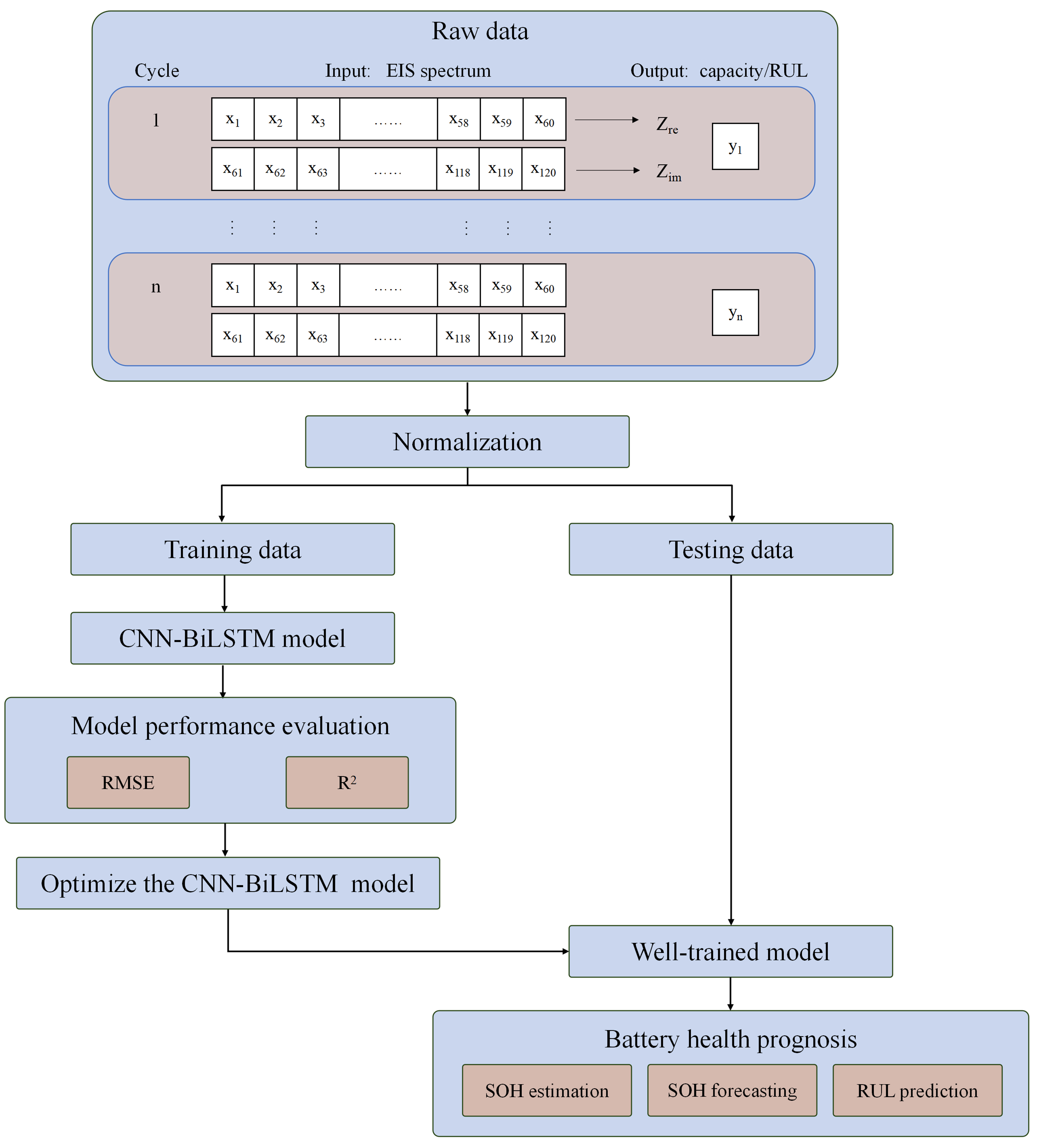
Figure 2. The flowchart of battery health prognosis via EIS using the CNN-BiLSTM model. The inputs to our model include both the real
SOH (current capacity) estimation
We first develop a CNN-BiLSTM model for capacity estimation using the EIS data from the current cycle, assuming a constant cycling temperature. The model is trained on five cells cycled at room temperature

Figure 3. SOH estimation and prediction at 25 °C. (A) Estimated (red curve) and measured (blue curve) capacity for the testing cell (marked as 25C05 in the EIS dataset). The coefficient of determination R2 of this model is displayed in the bottom left corner. Five-fold cross-validation was utilized to obtain a mean value derived from the outcomes of five distinct models which trained on 80% of the data and validated on the rest 20%; (B) Prediction of the capacity fade path (green curve). The red curve is the estimated capacity of the initial 50 cycles. Blue curve is the measured capacity for the 25C05 cell. The capacity is normalized relative to the initial capacity in each case. The shaded area in (A) and (B) plots indicates ±1 standard deviation. SOH: State of health; EIS: electrochemical impedance spectroscopy.
SOH (degradation trajectory) forecasting
Accurate prediction of the capacity degradation path is crucial for early detection of battery aging. Here, we propose the CNN-BiLSTM model to extrapolate the degradation trajectory for SOH forecasting. As shown in Figure 3B, the capacity of the initial 50 cycles is estimated from the EIS at each cycle (red curve), similar to the method used in Figure 3A. Moreover, the model effectively predicts the capacity (green curve) of a future cycle from 50 up to 300 by extrapolating the decreasing trend of the estimated capacity from the initial 50 cycles using the EIS data, revealing only a 17% (50 out of 300 cycles) degradation along the trajectory towards failure. The model provides a smoothed prediction of the gradual decrease in capacity during cycling. The narrow confidence intervals (orange-shaded region) in this plot indicate a higher degree of confidence in the accuracy of the predictions. These results demonstrate that the model successfully captures long-term degradation patterns in the EIS data. However, it should be noted that the model fails to predict the sudden decrease in capacity at cycle 190 [Figure 3A]. Forecasting such unexpected capacity fade at an early stage is a significant challenge due to the complex nature of battery failure mechanisms. Moreover, the prediction task is further complicated by the relatively small datasets (50 cycles) used, which cover a limited range of lifetimes. Nonetheless, we consider that this issue could be addressed by leveraging more comprehensive battery data from various aspects, such as in situ pressure and temperature measurements within the cell.
SOH estimation/forecasting at multiple temperatures
In the realm of battery recycling, forecasting battery health presents an even greater challenge, as historical operating conditions (e.g., temperature) vary across cells and cycles. It is highly desirable for a model to predict SOH based exclusively on EIS data from a given cycle, without requiring information about the cycling temperature except that it remains constant across cycles. To tackle this issue, we combine the training data collected at three different temperatures (i.e., five cells cycled at 25 °C, one cell each cycled at 35 and 45 °C), and retrain the CNN-BiLSTM models to learn features of the EIS dependent on capacity fade rather than temperature. The capacity curves of the training and testing sets for the multi-temperature models are shown in Supplementary Figures 4 and 5. Figure 4 shows that the multi-temperature models can accurately estimate current capacity and forecast the capacity degradation trajectory of cells cycled at 35 and 45 °C (marked as 35C02 and 45C02 in the EIS dataset).

Figure 4. SOH estimation and prediction at 35 and 45 °C. Estimated (red curve) and measured (blue curve) capacity for the testing cells 35C02 (A) and 45C02 (C). The R2 of this model is shown on the left bottom. Prediction of the capacity degradation trajectory (green curve) based on the EIS data from the initial 50 cycles. The blue curves represent the measured capacity for the 35C02 cell (B) and 45C02 cell (D). The capacity is normalized relative to the initial capacity in each case. The shaded area in all plots indicates ±1 standard deviation. SOH: State of health; EIS: electrochemical impedance spectroscopy.
Similarly, the multi-temperature CNN-BiLSTM model for capacity estimation also surpasses the GPR model, achieving higher R2 values of 0.85 and 0.80. Additionally, our model is compared with four other advanced predictive models, including LSTM, BiLSTM, and CNN-LSTM. In each comparison, our model consistently exhibits superior accuracy [Table 1]. We find that the R2 values of all five predictive models decrease as the temperature rises from 25 to 45 °C, suggesting that a more intense electrochemical process at higher temperatures may lead to less accurate capacity estimations. However, our multi-temperature models exhibit predictive robustness across various temperatures, as demonstrated by small RMSE values between 1.21 and 2.58 and narrow confidence intervals [Figure 4]. This verifies the value of the EIS-based approach for SOH estimation and forecasting of LIBs subjected to varying temperatures, which is crucial for practical applications where operating temperatures vary significantly across cells.
R2 values of different models in estimating SOH at various temperatures
| Model name | 25 °C | 35 °C | 45 °C |
| GPR1 | 0.88 | 0.81 | 0.72 |
| LSTM | 0.84 | 0.77 | 0.70 |
| BiLSTM | 0.87 | 0.78 | 0.68 |
| CNN-LSTM | 0.85 | 0.78 | 0.83 |
| CNN-BiLSTM | 0.89 | 0.84 | 0.80 |
RUL prediction at multiple temperatures
A key objective of a battery management system is to forecast the RUL of a battery and detect potentially hazardous conditions resulting from battery aging or misuse. Inspired by the approach of predicting SOH without temperature-specific information, we develop a multi-temperature model for predicting RUL using EIS data. Figure 5 shows the RUL forecasting results for test cells (marked as 25C01, 35C02 and 45C02) at three distinct temperatures (25, 35, and 45 °C). The multi-temperature CNN-BiLSTM model outperforms the other four models, achieving the highest R2 value for each case [Table 2]. The cycle count for RUL prediction is set in decreasing order from the end of life (when the capacity drops to 80% of its initial value) for each cell.

Figure 5. RUL prediction at three temperatures. Actual RUL and predicted RUL for (A) the 25C01 cell at 25 °C; (B) the 35C02 cell at
R2 values of different models in predicting RUL at various temperatures
| Model name | 25 °C | 35 °C | 45 °C |
| GPR1 | 0.87 | 0.75 | 0.92 |
| LSTM | 0.61 | 0.86 | 0.76 |
| BiLSTM | 0.79 | 0.83 | 0.79 |
| CNN-LSTM | 0.74 | 0.85 | 0.84 |
| CNN-BiLSTM | 0.85 | 0.86 | 0.94 |
Overall, the CNN-BiLSTM model shows remarkable efficiency in interpreting high-dimensional impedance spectra for both SOH estimation and RUL forecasting of batteries. This is attributed to its integration of both CNNs and LSTM networks, enabling the model to effectively utilize spatial patterns for recognizing quantitative changes in EIS spectra and temporal sequences for modeling degradation across cycles simultaneously. Additionally, the bidirectional nature of the BiLSTM allows the model to incorporate past and future information on EIS data when making predictions, thereby enhancing its predictive performance in battery health prognosis. It is worth noting, however, that the predictive performance of models may vary across different test cells due to capacity inconsistency originating from manufacturing processes.
CONCLUSIONS
In this paper, we develop versatile CNN-BiLSTM models for accurate battery health prognosis using EIS spectra from LIBs exhibiting various degradation patterns under different cycling temperatures. The models demonstrate enhanced precision in estimating current capacity, even in the face of sudden drops, and in predicting the RUL compared to the earlier state-of-the-art Gaussian Process method. Moreover, our model, for the first time, enables the forecast of long-term battery degradation trajectory toward failure based on a limited set of early-cycle EIS data. This capability holds significant potential for early-lifetime safety warning of LIBs. Leveraging the capabilities of CNN and BiLSTM models, our CNN-BiLSTM model consistently outperforms the previous state-of-the-art GPR model and other existing predictive models, such as CNN, LSTM and BiLSTM. Thus, our work identifies that both spatial and temporal features of EIS spectra correlate with degradation patterns and play an important role in accurate battery prognosis. We showcase the potential implementation of our EIS-based CNN-BiLSTM model in battery management systems to address health prediction under realistic operating conditions, including variations in cycling temperature over time and fluctuations in charge/discharge rates.
DECLARATIONS
Authors’ contributions
Conceptualization: Zhang Y, Liu Z, Sun Y, Liu Y
Methodology, software, validation, formal analysis and data curation: Li Y
Investigation, write - original draft, write - review and editing and visualization: Sun Y, Li Y
Project administration and funding acquisition: Zhang Y, Chen Y
Supervision: Zhang Y, Liu Y, Chen Y
Availability of data and materials
The code is available from the GitHub link at https://github.com/YunweiZhang1/Battery-health-prediction-CNN-BiLSTM.
Financial support and sponsorship
Zhang Y acknowledges funding from the National Key Research and Development Program of China (2023YFB3001704), National Natural Science Foundation of China (Grant No. 12304036), the Open Project of Guangdong Provincial Key Laboratory of Magnetoelectric Physics and Devices (No. 2022B1212010008), the Guangdong Basic and Applied Basic Research Foundation (2023A1515010071), the Guangzhou Basic and Applied Basic Research Foundation (SL2022A04J00048), and the Fundamental Research Funds for the Central Universities, Sun Yat-sen University (23xkjc016). Chen Y is grateful for the financial support from the Research Grants Council of Hong Kong (C7002-22Y) and the research computing facilities offered by ITS, HKU.
Conflicts of interest
Sun Y and Liu Y are affiliated with DeepVerse PTE. LTD, while the other authors have declared that they have no conflicts of interest.
Ethical approval and consent to participate
Not applicable.
Consent for publication
Not applicable.
Copyright
© The Author(s) 2024.
Supplementary Materials
REFERENCES
1. Harper G, Sommerville R, Kendrick E, et al. Recycling lithium-ion batteries from electric vehicles. Nature 2019;575:75-86.
2. Zubi G, Dufo-lópez R, Carvalho M, Pasaoglu G. The lithium-ion battery: state of the art and future perspectives. Renew Sust Energ Rev 2018;89:292-308.
3. Lu L, Han X, Li J, Hua J, Ouyang M. A review on the key issues for lithium-ion battery management in electric vehicles. J Power Sources 2013;226:272-88.
4. Yang S, Zhang C, Jiang J, Zhang W, Zhang L, Wang Y. Review on state-of-health of lithium-ion batteries: characterizations, estimations and applications. J Clean Prod 2021;314:128015.
5. Liu W, Placke T, Chau K. Overview of batteries and battery management for electric vehicles. Energy Rep 2022;8:4058-84.
6. Chen Y, Kang Y, Zhao Y, et al. A review of lithium-ion battery safety concerns: the issues, strategies, and testing standards. J Energy Chem 2021;59:83-99.
7. Xu B, Oudalov A, Ulbig A, Andersson G, Kirschen DS. Modeling of lithium-ion battery degradation for cell life assessment. IEEE Trans Smart Grid 2018;9:1131-40.
8. Li J, Adewuyi K, Lotfi N, Landers R, Park J. A single particle model with chemical/mechanical degradation physics for lithium ion battery state of health (SOH) estimation. Appl Energy 2018;212:1178-90.
9. Neupert S, Kowal J. Model-based state-of-charge and state-of-health estimation algorithms utilizing a new free lithium-ion battery cell dataset for benchmarking purposes. Batteries 2023;9:364.
10. Li J, Landers R, Park J. A comprehensive single-particle-degradation model for battery state-of-health prediction. J Power Sources 2020;456:227950.
11. Maheshwari A, Paterakis NG, Santarelli M, Gibescu M. Optimizing the operation of energy storage using a non-linear lithium-ion battery degradation model. Appl Energy 2020;261:114360.
12. Pender JP, Jha G, Youn DH, et al. Electrode degradation in lithium-ion batteries. ACS Nano 2020;14:1243-95.
13. Birkl CR, Roberts MR, Mcturk E, Bruce PG, Howey DA. Degradation diagnostics for lithium ion cells. J Power Sources 2017;341:373-86.
14. Zhang M, Yang D, Du J, et al. A review of SOH prediction of Li-ion batteries based on data-driven algorithms. Energies 2023;16:3167.
15. Lombardo T, Duquesnoy M, El-Bouysidy H, et al. Artificial intelligence applied to battery research: hype or reality? Chem Rev 2022;122:10899-969.
16. Deng Z, Lin X, Cai J, Hu X. Battery health estimation with degradation pattern recognition and transfer learning. J Power Sources 2022;525:231027.
17. Khaleghi S, Karimi D, Beheshti SH, et al. Online health diagnosis of lithium-ion batteries based on nonlinear autoregressive neural network. Appl Energy 2021;282:116159.
18. Hossain Lipu M, Ansari S, Miah MS, et al. Deep learning enabled state of charge, state of health and remaining useful life estimation for smart battery management system: methods, implementations, issues and prospects. J Energy Storage 2022;55:105752.
19. Jones PK, Stimming U, Lee AA. Impedance-based forecasting of lithium-ion battery performance amid uneven usage. Nat Commun 2022;13:4806.
20. Severson KA, Attia PM, Jin N, et al. Data-driven prediction of battery cycle life before capacity degradation. Nat Energy 2019;4:383-91.
21. Che Y, Hu X, Lin X, Guo J, Teodorescu R. Health prognostics for lithium-ion batteries: mechanisms, methods, and prospects. Energy Environ Sci 2023;16:338-71.
22. Li C, Xiao F, Fan Y. An approach to state of charge estimation of lithium-ion batteries based on recurrent neural networks with gated recurrent unit. Energies 2019;12:1592.
23. Xu Z, Wang J, Fan Q, Lund PD, Hong J. Improving the state of charge estimation of reused lithium-ion batteries by abating hysteresis using machine learning technique. J Energy Storage 2020;32:101678.
24. Peng K, Deng Z, Bao Z, Hu X. Data-driven battery capacity estimation based on partial discharging capacity curve for lithium-ion batteries. J Energy Storage 2023;67:107549.
25. Zheng L, Zhu J, Lu DD, Wang G, He T. Incremental capacity analysis and differential voltage analysis based state of charge and capacity estimation for lithium-ion batteries. Energy 2018;150:759-69.
26. Fei Z, Yang F, Tsui K, Li L, Zhang Z. Early prediction of battery lifetime via a machine learning based framework. Energy 2021;225:120205.
27. Shu X, Shen S, Shen J, et al. State of health prediction of lithium-ion batteries based on machine learning: advances and perspectives. iScience 2021;24:103265.
28. Choi W, Shin H, Kim JM, Choi J, Yoon W. Modeling and applications of electrochemical impedance spectroscopy (EIS) for lithium-ion batteries. J Electrochem Sci Technol 2020;11:1-13.
29. Meddings N, Heinrich M, Overney F, et al. Application of electrochemical impedance spectroscopy to commercial Li-ion cells: a review. J Power Sources 2020;480:228742.
30. Middlemiss LA, Rennie AJ, Sayers R, West AR. Characterisation of batteries by electrochemical impedance spectroscopy. Energy Rep 2020;6:232-41.
31. Juarez-robles D, Chen C, Barsukov Y, P. Mukherjee P. Impedance evolution characteristics in lithium-ion batteries. J Electrochem Soc 2017;164:A837-47.
32. Gaberšček M. Understanding Li-based battery materials via electrochemical impedance spectroscopy. Nat Commun 2021;12:6513.
33. Moradighadi N, Nesic S, Tribollet B. Identifying the dominant electrochemical reaction in electrochemical impedance spectroscopy. Electrochim Acta 2021;400:139460.
34. Li D, Yang D, Li L, Wang L, Wang K. Electrochemical impedance spectroscopy based on the state of health estimation for lithium-ion batteries. Energies 2022;15:6665.
35. Jiang B, Zhu J, Wang X, Wei X, Shang W, Dai H. A comparative study of different features extracted from electrochemical impedance spectroscopy in state of health estimation for lithium-ion batteries. Appl Energy 2022;322:119502.
36. Zhang Y, Tang Q, Zhang Y, Wang J, Stimming U, Lee AA. Identifying degradation patterns of lithium ion batteries from impedance spectroscopy using machine learning. Nat Commun 2020;11:1706.
37. Lecun Y, Bottou L, Bengio Y, Haffner P. Gradient-based learning applied to document recognition. Proc IEEE 1998;86:2278-324.
38. Rumelhart DE, Hinton GE, Williams RJ. Learning representations by back-propagating errors. Nature 1986;323:533-6.
40. Graves A, Schmidhuber J. Framewise phoneme classification with bidirectional LSTM and other neural network architectures. Neural Netw 2005;18:602-10.
41. Koroma MS, Costa D, Philippot M, et al. Life cycle assessment of battery electric vehicles: implications of future electricity mix and different battery end-of-life management. Sci Total Environ 2022;831:154859.
Cite This Article
Export citation file: BibTeX | EndNote | RIS
OAE Style
Liu Z, Sun Y, Li Y, Liu Y, Chen Y, Zhang Y. Lithium-ion battery health prognosis via electrochemical impedance spectroscopy using CNN-BiLSTM model. J Mater Inf 2024;4:9. http://dx.doi.org/10.20517/jmi.2024.09
AMA Style
Liu Z, Sun Y, Li Y, Liu Y, Chen Y, Zhang Y. Lithium-ion battery health prognosis via electrochemical impedance spectroscopy using CNN-BiLSTM model. Journal of Materials Informatics. 2024; 4(2): 9. http://dx.doi.org/10.20517/jmi.2024.09
Chicago/Turabian Style
Zhihang Liu, Yi Sun, Yutian Li, Yuyang Liu, Yue Chen, Yunwei Zhang. 2024. "Lithium-ion battery health prognosis via electrochemical impedance spectroscopy using CNN-BiLSTM model" Journal of Materials Informatics. 4, no.2: 9. http://dx.doi.org/10.20517/jmi.2024.09
ACS Style
Liu, Z.; Sun Y.; Li Y.; Liu Y.; Chen Y.; Zhang Y. Lithium-ion battery health prognosis via electrochemical impedance spectroscopy using CNN-BiLSTM model. J. Mater. Inf. 2024, 4, 9. http://dx.doi.org/10.20517/jmi.2024.09
About This Article
Special Issue
Copyright

Data & Comments
Data
0


Comments
Comments must be written in English. Spam, offensive content, impersonation, and private information will not be permitted. If any comment is reported and identified as inappropriate content by OAE staff, the comment will be removed without notice. If you have any queries or need any help, please contact us at support@oaepublish.com.